Machine Learning with Python Cookbook 学习笔记第12章_dict(c=para.c,kernel=para.kernel,gamma=para.gamma)-优快云博客

本文链接：https://blog.youkuaiyun.com/weixin_51083297/article/details/125941794

Chapter 12. Model Selection

前言

本笔记是针对人工智能典型算法的课程中Machine Learning with Python Cookbook的学习笔记
学习的实战代码都放在代码压缩包中
实战代码的运行环境是python3.9 numpy 1.23.1 **anaconda 4.12.0 **
上一章：(97条消息) Machine Learning with Python Cookbook 学习笔记第11章_五舍橘橘的博客-优快云博客
代码仓库
- Github:yy6768/Machine-Learning-with-Python-Cookbook-notebook: 人工智能典型算法笔记 (github.com)
- Gitee:yyorange/机器学习笔记代码仓库 (gitee.com)

12.0 Introduction

在机器学习中，我们使用训练算法通过最小化一些损失函数来学习模型的参数。除此之外，许多学习算法（例如，支持向量分类器和随机森林）也有必须在学习过程之外定义的超参数（hyperparameters）。
我们通常可能想尝试多种学习算法（例如，同时尝试支持向量分类器和随机森林，看看哪种学习方法产生了最好的模型）。
我们将选择最佳学习算法及其最佳超参数都称为模型选择。
在本章中，我们将介绍从候选集中有效地选择最佳模型的技术。
在本章中，我们将参考特定的超参数。，例如 C（正则化强度的倒数）。

12.1 Selecting Best Models Using Exhaustive Search

通过穷举法来找出最好的模型
GridSearchCV

exhaustiveSearch.py

# Load libraries
import numpy as np
from sklearn import linear_model, datasets
from sklearn.model_selection import GridSearchCV

# 莺尾花数据
iris = datasets.load_iris()
features = iris.data
target = iris.target
# 创建 logistic regression
logistic = linear_model.LogisticRegression()
# 创造超参数-regularization penalty的可能的序列
penalty = ['l1', 'l2']
# 创建C的可能的序列
C = np.logspace(0, 4, 10)  # np.logspace生成等比数列
# 创建一个字典，C和penalty分别指向两个参数
hyperparameters = dict(C=C, penalty=penalty)
# 查看参数信息
print(hyperparameters)
# 进行穷举搜索
gridsearch = GridSearchCV(logistic, hyperparameters, cv=5, verbose=0)
# fit最佳模型
best_model = gridsearch.fit(features, target)

Discussion

GridSearchCV 是一种使用交叉验证进行模型选择的暴力方法。
- 用户为一个或多个超参数定义一组可能的值，然后 GridSearchCV 使用每个值和/或值的组合训练模型。
- 选择性能得分最高的模型作为最佳模型。
解析一下我们代码是怎么寻找到最佳模型
- 在我们的解决方案中，我们使用逻辑回归（LogisticRegression）（将在接下来的章节介绍，所以并不需要掌握C和正则化惩罚参数是什么，只需要知道他们是超参数）作为我们的模型
- 逻辑回归拥有两个超参数：
  - C
  - regularization penalty
- 对于我们的C我们使用numpy的logspace创建了一组等比数列
```
np.logspace(0, 4, 10)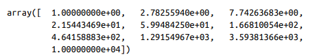
```
- 同样我们也定义了两个正则化惩罚可能的值：[l1,l2]
- 检验方法我们选择的是k值为5的k折交叉检验法
- 而GridSearchCV暴力的创建了10（C值的个数）× 2（正则化惩罚的个数）×5（k折交叉检验）个候选模型，从这100个模型里选择出评估得分最高的
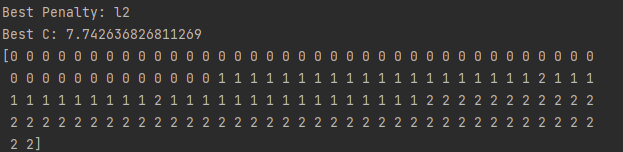
- 我们可以查看最好模型的超参数，并且使用它进行预测：
```
# 查看超参数
print('Best Penalty:', best_model.best_estimator_.get_params()['penalty'])
print('Best C:', best_model.best_estimator_.get_params()['C'])
# 预测
print(best_model.predict(features))
```

GridSearchCV的参数：
- verbose：最值得注意的一个参数：verbose 参数决定了搜索过程中输出的消息量，0 表示没有输出，1 到 3 表示输出的消息越来越详细
- cv：交叉检验法
- n_job、scoring和之前的参数一样
- api:sklearn.model_selection.GridSearchCV — scikit-learn 1.1.1 documentation

12.2 Selecting Best Models Using Randomized Search

对模型进行随机搜索
RandomizedSearchCV

randomizedSearch.py

# Load libraries
from scipy.stats import uniform
from sklearn import linear_model, datasets
from sklearn.model_selection import RandomizedSearchCV

# 加载莺尾花
iris = datasets.load_iris()
features = iris.data
target = iris.target
# 逻辑回归
logistic = linear_model.LogisticRegression()
# 惩罚项可能的值
penalty = ['l1', 'l2']
# C可能的值
C = uniform(loc=0, scale=4)  # 随机数生成C
# 创建超参数字典供searchCv选择
hyperparameters = dict(C=C, penalty=penalty)
# 随机化搜索
randomizedsearch = RandomizedSearchCV(
    logistic, hyperparameters, random_state=1, n_iter=100, cv=5, verbose=0,
    n_jobs=-1)
# 选择出最好的模型并训练
best_model = randomizedsearch.fit(features, target)

Discussion

RandomizedSearchCV的原理是从用户提供的分布（例如，正态分布、均匀分布）中搜索特定数量的超参数值的随机组合。
如果我们指定一个分布，scikit-learn 将随机抽样而不像GridSearchCV从该分布中替换超参数值。
- 本示例中，我们从 0 到 4 的均匀分布中随机抽取 10 个值作为C的候选序列：
- 我们和上一节一样，以[l1,l2]作为惩罚项的候选序列，但是本例中RandomizedSearchCV不是生成更多的模型，而是对两者进行随机的抽样
像使用 GridSearchCV 一样，我们可以看到最佳模型的超参数值：

最佳模型也可以进行预测

# 查看超参数
print('Best Penalty:', best_model.best_estimator_.get_params()['penalty'])
print('Best C:', best_model.best_estimator_.get_params()['C'])

# 预测目标
best_model.predict(features)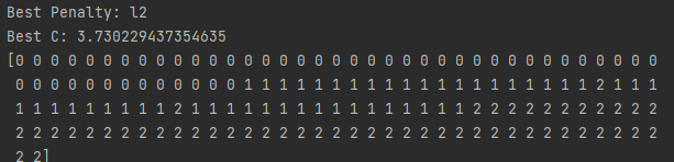

超参数的采样组合的数量（即训练的候选模型的数量）由 n_iter（迭代次数）设置指定。
api:sklearn.model_selection.RandomizedSearchCV — scikit-learn 1.1.1 documentation

12.3 Selecting Best Models from Multiple Learning Algorithms

从多种学习算法中选择出最佳模型
建立一个包含多种学习算法和它们各自的参数的字典

multiAlgorithm.py

# Load libraries
import numpy as np
from sklearn import datasets
from sklearn.linear_model import LogisticRegression
from sklearn.ensemble import RandomForestClassifier
from sklearn.model_selection import GridSearchCV
from sklearn.pipeline import Pipeline

# 创建随机数种子
np.random.seed(0)
# 加载莺尾花数据集
iris = datasets.load_iris()
features = iris.data
target = iris.target
# 创建一个管道进行训练优化
pipe = Pipeline([("classifier", RandomForestClassifier())])
# 创建一个字典，包含学习算法数组和他们的参数
search_space = [{"classifier": [LogisticRegression()],  # 逻辑回归
                 "classifier__penalty": ['l1', 'l2'],
                 "classifier__C": np.logspace(0, 4, 10)},
                {"classifier": [RandomForestClassifier()],  # 随机森林
                 "classifier__n_estimators": [10, 100, 1000],
                 "classifier__max_features": [1, 2, 3]}]
# 穷举搜索和cv交叉检验评估
gridsearch = GridSearchCV(pipe, search_space, cv=5, verbose=0)
# 选择出的模型进行训练
best_model = gridsearch.fit(features, target)

Discussion

我们可以通过字典扩大搜索空间，从而实现从多种学习算法中选择
本例中我们在LogisticRegression和RandomForestClassifier中进行选择

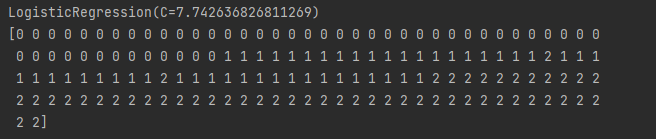
搜索结束后可以查看选择的最佳模型的学习算法，超参数等信息

# 查看模型
print(best_model.best_estimator_.get_params()["classifier"])
# 进行预测
print(best_model.predict(features))

12.4 Selecting Best Models When Preprocessing

在模型选择的过程中进行数据预处理
创建pipeline并将预处理加入到pipeline中

preprocessing.py

# Load libraries
import numpy as np
from sklearn import datasets
from sklearn.linear_model import LogisticRegression
from sklearn.model_selection import GridSearchCV
from sklearn.pipeline import Pipeline, FeatureUnion
from sklearn.decomposition import PCA
from sklearn.preprocessing import StandardScaler

# 随机数种子
np.random.seed(0)
# 加载莺尾花数据集
iris = datasets.load_iris()
features = iris.data
target = iris.target
# 预处理包括预处理和PCA降维
preprocess = FeatureUnion([("std", StandardScaler()), ("pca", PCA())])
# 创建一个管道包含预处理和模型选择
pipe = Pipeline([("preprocess", preprocess),
                 ("classifier", LogisticRegression())])
# PCA参数的搜索空间和超参数的搜索空间
search_space = [{"preprocess__pca__n_components": [1, 2, 3],
                 "classifier__penalty": ["l1", "l2"],
                 "classifier__C": np.logspace(0, 4, 10)}]
# 暴力搜索
clf = GridSearchCV(pipe, search_space, cv=5, verbose=0, n_jobs=-1)
# 训练
best_model = clf.fit(features, target)

Discussion

很多时候，我们需要在使用它来训练模型之前对数据进行预处理。
在进行模型选择时，我们必须小心正确地处理预处理.
- 首先，GridSearchCV 使用交叉验证来确定哪个模型具有最高性能.
- 在交叉验证中，我们实际上是在假装折叠保持不变，因为没有看到测试集，因此不是拟合任何预处理步骤（例如，缩放或标准化）的一部分。出于这个原因，我们不能预处理数据然后运行 GridSearchCV。
FeatureUnion 允许我们正确地组合多个预处理操作。在我们的解决方案中，我们使用 FeatureUnion 来组合两个预处理步骤：标准化特征值（StandardScaler(第4章)）和主成分分析（PCA（第9章））。
我们使用我们的学习算法将预处理包含到管道中。最终结果是，这使我们能够将使用超参数组合的模型的拟合、转换和训练的正确（和令人困惑的）处理外包给 scikit-learn。
一些预处理方法有自己的参数，这些参数通常必须由用户提供。例如，使用 PCA 进行降维需要用户定义用于生成转换特征集的主成分的数量。scikit-learn 让这一切变得简单。当我们在搜索空间中包含候选组件值时，它们被视为要搜索的任何其他超参数。

模型选择完成后，我们可以查看产生最佳模型的预处理值。

# 最佳模型的PCA特征数量
print(best_model.best_estimator_.get_params()['preprocess__pca__n_components'])

12.5 Speeding Up Model Selection with Parallelization

加速模型选择
n_jobs=-1

speedingUp.py

# Load libraries

import numpy as np
from sklearn import linear_model, datasets
from sklearn.model_selection import GridSearchCV
import datetime
starttime = datetime.datetime.now()


# 加载数据集
iris = datasets.load_iris()
features = iris.data
target = iris.target
# 逻辑回归
logistic = linear_model.LogisticRegression()
# penalty超参数候选值
penalty = ["l1", "l2"]
# C候选值
C = np.logspace(0, 4, 1000)
# 创建超参数搜索空间
hyperparameters = dict(C=C, penalty=penalty)
# 暴力搜索
gridsearch = GridSearchCV(logistic, hyperparameters, cv=5, n_jobs=-1, verbose=1)
# 训练模型
best_model = gridsearch.fit(features, target)

endtime = datetime.datetime.now()
print((endtime-starttime).seconds)

运行48s

将n_jobs改为1

时间为155s

Discussion

在现实世界中，我们通常会有数千或数万个模型需要训练。最终结果是找到最佳模型可能需要花费数小时
为了加快这个过程，scikit-learn 让我们可以同时训练多个模型。在不涉及太多技术细节的情况下，scikit-learn 可以同时训练模型达到机器上的核心数量。
参数 n_jobs 定义要并行训练的模型数量。在我们的解决方案中，我们将 n_jobs 设置为 -1，这告诉 scikit-learn 使用所有内核。
默认情况下 n_jobs 设置为 1，这意味着它只使用一个核心。

12.6 Speeding Up Model Selection Using Algorithm-Specific Methods

和上一节的目标一样，我们需要加速模型选择
假设需要在特定的学习方法中选择模型，使用 scikit-learn中模型交叉验证的超参数进行调整。

例如LogisticRegressionCV:

specificMethods.py

# Load libraries
from sklearn import linear_model, datasets
# Load data
iris = datasets.load_iris()
features = iris.data
target = iris.target
# Create cross-validated logistic regression
logit = linear_model.LogisticRegressionCV(Cs=100)
# Train model
print(logit.fit(features, target))

Discussion

在 scikit-learn 中，许多学习算法（例如 Ridge回归、lasso回归和elastic net regression（弹性网络回归算法））都有一种特定于该算法的交叉验证方法
- 例如，LogisticRegression 用于进行标准逻辑回归分类器，而 LogisticRegressionCV 实现了一个高效的交叉验证逻辑回归分类器，能够识别超参数 C 的最佳值。
- 参数CS:C的一系列候选值
  - 如果是列表，则Cs作为一个超参数，列表中的值是Cs的候选值
  - 如果提供列表，则 Cs 是要从中选择的候选超参数值。
  - 候选值是从 0.0001 到 1,0000 之间的范围（C 的合理值范围）以对数方式得出的。
- LogisticRegressionCV 的一个主要缺点是它只能搜索 C 的一系列值。在 12.1 节中，我们可能的超参数空间包括 C 和另一个超参数（正则化惩罚范数）。
  
  这样无法照顾到全部超参数的限制在 scikit-learn 的许多特定于模型的交叉验证方法中很常见

scikit-learn常见的特定交叉验证方法：

3.2. Tuning the hyper-parameters of an estimator — scikit-learn 1.1.1 documentation

12.7 Evaluating Performance After Model Selection

在选择模型之后评估模型的质量
使用嵌套的交叉验证评估来避免评估具有偏差

evaluateAfterSelecting.py

# Load libraries
import numpy as np
from sklearn import linear_model, datasets
from sklearn.model_selection import GridSearchCV, cross_val_score
# 加载数据
iris = datasets.load_iris()
features = iris.data
target = iris.target
# 逻辑回归
logistic = linear_model.LogisticRegression()
# 创建20个候选的C值
C = np.logspace(0, 4, 20)
# 可选择的超参数的代数空间
hyperparameters = dict(C=C)
# 穷举搜索
gridsearch = GridSearchCV(logistic, hyperparameters, cv=5, n_jobs=-1, verbose=0)
# 嵌套的交叉检验计算的出平均值
print(cross_val_score(gridsearch, features, target).mean())

Discussion

由于我们已经使用了交叉检验来产生了最佳的模型，但是如果我们还使用同样的数据来进行评估的话，结果明显是不可靠的。
因此产生了嵌套交叉检验的方法。“内部”交叉验证选择最佳模型，而“外部”交叉验证为我们提供了对模型性能的无偏见评估。
在我们的解决方案中，内部交叉验证是我们的GridSearchCV对象，然后我们使用 cross_val_score 将其包装在外部交叉验证中。
可能这样比较晦涩，在前几节中我们学习了verbose参数可以控制输出的信息。
- 我们使用verbose=1：
```
gridsearch = GridSearchCV(logistic, hyperparameters, cv=5, n_jobs=-1, verbose=1)
```
- 运行训练最佳模型的fit，生成一条信息（内部交叉检验产生的）
```
# 查看嵌套时的信息
# 内部
best_model = gridsearch.fit(features, target)
```
  得到结果：
- 运行cross_val_score:
```
# 外部
scores = cross_val_score(gridsearch, features, target)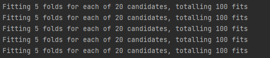
```
生成的结果可以看到内部的CV又训练了5次100的模型
- 我们可以从结果中看出，cross_val_score需要进行五折交叉检验（原书为旧版本scikit-learn,默认为3折)，然后内层的每次需要进行5折的交叉检验，所以嵌套的交叉检验总共要进行20*5*5=500次训练