Machine Learning with Python Cookbook 学习笔记 第4章

Chapter 4 Handling Numerical Data

前言

• 本笔记是针对人工智能典型算法的课程中Machine Learning with Python Cookbook的学习笔记

• 学习的实战代码都放在代码压缩包中

• 实战代码的运行环境是python3.9 numpy 1.23.1
  上一章：(89条消息) Machine Learning with Python Cookbook 学习笔记 第3章_五舍橘橘的博客-优快云博客

4.0 Introduction

Quantitative data is the measurment of something–weather class size, monthly sales, or student scores. The natural way to represent these quantities is numerically (e.g., 20 students, $529,392 in sales). In this chapter we will cover numerous strategies for transforming raw numerical data into features purpose-built for machine learning algoristshms

• 在本章中，我们将介绍许多将原始数值数据转换为专为机器学习算法构建的特征的策略

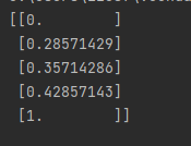
4.1 Rescaling a feature

Use scikit-learn’s MinMaxScaler to rescale a feature array

特征缩放是什么？特征缩放的目标就是数据规范化，使得特征的范围具有可比性。它是数据处理的预处理处理，对后面的使用数据具有关键作用。

rescalingExample.py

# Load libraries
import numpy as np
from sklearn import preprocessing

# 创建特征矩阵
feature = np.array([[-500.5],
                    [-100.1],
                    [0],
                    [100.1],
                    [900.9]])
# Create scaler
minmax_scale = preprocessing.MinMaxScaler(feature_range=(0, 1))
# Scale feature
scaled_feature = minmax_scale.fit_transform(feature)
# Show feature
print(scaled_feature)

Discussion

Discussion

Rescaling is a common preprocessing task in machine learning. Many of the algorithms described later in this book will assume all features are on the same scale, typically 0 to 1 or -1 to 1. There are a number of rescaling techniques, but one of the simlest is called min-max scaling. Min-max scaling uses the minimum and maximum values of a feature to rescale values to within a range. Specfically, min-max calculates:

• 特征缩放是机器学习中常见的预处理任务。
• 本书后面描述的许多算法将假设所有特征都处于相同的比例，通常是 0 到 1 或 -1 到 1。有许多重新缩放技术
• 本节使用的是最简单的一种称为min-max scaling的技术

$$x_i‘=\frac{x_i-min(x)}{max(x)-min(x)}$$

where x is the feature vector, $x_i$ is an individual element of feature x, and $x_i^{‘}$ is the rescaled element

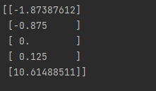
4.2 Standardizing a Feature

scikit-learn’s StandardScaler transforms a feature to have a mean of 0 and a standard deviation of 1.

standardScalerExample.py

import numpy as np
from sklearn import preprocessing

feature = np.array([
    [-1000.1],
    [-200.2],
    [500.5],
    [600.6],
    [9000.9]
])

scaler = preprocessing.StandardScaler()

# 标准化
standardized = scaler.fit_transform(feature)

print(standardized)

[外链图片转存失败,源站可能有防盗链机制,建议将图片保存下来直接上传(img-jGo05LvF-1658046689642)(C:\Users\12587\AppData\Roaming\Typora\typora-user-images\image-20220715152805484.png)]

Discussion

• 标准化使的feature的均值 $\bar{x}$为0，$\sigma$为1
• $$x_i^{‘}=\frac{x_i-\bar{x}}{\sigma }$$
• 标准化是机器学习预处理的常用缩放方法，比最大最小化法用的多。但是还是建议在神经网络中使用最大最小化法，不使用标准化
• 如果我们的数据有明显的异常值，它会通过影响特征的均值和方差来对我们的标准化产生负面影响。在这种情况下，使用中位数和四分位数范围重新调整特征通常会有所帮助。在 scikit-learn 中，我们使用 RobustScaler 方法执行此操作：

import numpy as np
from sklearn import preprocessing

feature = np.array([
    [-1000.1],
    [-200.2],
    [500.5],
    [600.6],
    [9000.9]
])

# scaler = preprocessing.StandardScaler()
#
# # 标准化
# standardized = scaler.fit_transform(feature)
#
# print(standardized)

# create scaler
robust_scaler = preprocessing.RobustScaler()

# 中值代替
robust = robust_scaler.fit_transform(feature)

print(robust)

4.3 Normalizing Observations

Use scikit-learn’s Normalizer to rescale the feature values to have unit norm (a total length of 1)

observationNormalizeExample.py

import numpy as np
from sklearn.preprocessing import Normalizer

# create feature matrix
features = np.array([
    [0.5, 0.5],
    [1.1, 3.4],
    [1.5, 20.2],
    [1.63, 34.4],
    [10.9, 3.3]
])

# create normalizer
normalizer = Normalizer(norm="l2")

# normalize matrix
print(normalizer.transform(features))

[外链图片转存失败,源站可能有防盗链机制,建议将图片保存下来直接上传(img-n3kYJJUs-1658046689643)(C:\Users\12587\AppData\Roaming\Typora\typora-user-images\image-20220715160050862.png)]

Discussion

• Normalizer 根据参数将单个观测值的值重新调整为具有单位的范式（它们的长度之和为 1）。

• Normalizer 提供了三个范式选项，欧几里得范数（通常称为 L2）是默认值： $$||x|{|}_2=\sqrt{x_1^2+x_2^2+...+x_n^2}$$

• 曼哈顿范数 (L1)： $$||x|{|}_1=\sum _{i=1}^n{x}_i$$

• 实际上，请注意 norm='l1' 会重新调整观察值，使其总和为 1，这有时可能是理想的质量

# transform feature matrix
features_l1_norm = Normalizer(norm="l1").transform(features)
print("Sum of the first observation's values: {}".format(features_l1_norm[0,0] + features_l1_norm[0,1]))

结果：Sum of the first observation’s values: 1.0

• 查寻资料得到第三种参数为max,若为max时，样本各个特征值除以样本中特征值最大的值

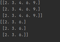
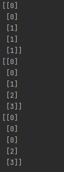
4.4 Generating Polynomial and Interaction Features

Problem

创建多项式特征

Solution

使用scikit-learn里的built-in函数

polynomialExample.py

# Load libraries
import numpy as np
from sklearn.preprocessing import PolynomialFeatures

# Create feature matrix
features = np.array([[2, 3],
                     [2, 3],
                     [2, 3]])
# Create PolynomialFeatures object
polynomial_interaction = PolynomialFeatures(degree=2, include_bias=False)
# 创建多项式特征
print(polynomial_interaction.fit_transform(features))

# 只出现交叉项
interaction = PolynomialFeatures(degree=2,
                                 interaction_only=True, include_bias=False)
print(interaction.fit_transform(features))

Discussion

• 什么是多项式特征？为什么要创建多项式特征

  多项式特征可以理解成现有特征的乘积。当我们想要包含特征与目标之间存在非线性关系的概念时，通常会创建多项式特征。

• 此外，我们经常会遇到一个特性的效果依赖于另一个特性的情况。每个特征对目标（甜度）的影响是相互依赖的。我们可以通过包含一个交互特征来对这种关系进行编码，该交互特征是各个特征的产物。

4.5 Transforming Features

对一组特征进行自定义的转换

在 scikit-learn 中，使用 FunctionTransformer 将函数应用于一组 特征：

transformingExample.py

# Load libraries
import numpy as np
from sklearn.preprocessing import FunctionTransformer

# Load library
import pandas as pd

# Create feature matrix
features = np.array([[2, 3],
                     [2, 3],
                     [2, 3]])


# 创建一个函数
def add_ten(x):
    return x + 10


# Create transformer
ten_transformer = FunctionTransformer(add_ten)
# 运用transformer
print(ten_transformer.transform(features))


# 将features创建为DataFrame
df = pd.DataFrame(features, columns=["feature_1", "feature_2"])
# 使用第三章的apply函数
df.apply(add_ten)

[外链图片转存失败,源站可能有防盗链机制,建议将图片保存下来直接上传(img-KDGkcpeK-1658046689644)(C:\Users\12587\AppData\Roaming\Typora\typora-user-images\image-20220715170752238.png)]

Discussion

• 通常希望对一项或多项功能进行一些自定义转换。
• add_ten是一个很简单的函数，但是实际应用种我们可以使用transformer或者apply进行更复杂的函数的应用

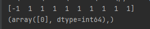
4.6 Detecting Outliers

检测异常值

detectOutliersExample.py

# Load libraries
import numpy as np
from sklearn.covariance import EllipticEnvelope
from sklearn.datasets import make_blobs

# 创建模拟值
features, _ = make_blobs(n_samples=10,
                         n_features=2,
                         centers=1,
                         random_state=1)
# 将第一行的值替换为一个极端的值
features[0, 0] = 10000
features[0, 1] = 10000
# 创建一个detector
outlier_detector = EllipticEnvelope(contamination=.1)
# 拟合 detector
outlier_detector.fit(features)
# 预测 outliers
print(outlier_detector.predict(features))


# 创建 单一 feature
feature = features[:, 0]

# 创建函数计算iqr并且返回iqr外的值
def indicies_of_outliers(x):
    q1, q3 = np.percentile(x, [25, 75])
    iqr = q3 - q1
    lower_bound = q1 - (iqr * 1.5)
    upper_bound = q3 + (iqr * 1.5)
    return np.where((x > upper_bound) | (x < lower_bound))


# Run function
print(indicies_of_outliers(feature))

结果：

本案例主要展现两种检测异常值的方法

EllipticEnvelope

• 假设全部数据可以表示成基本的多元高斯分布（正态分布），EllipticEnvelope函数试图找出数据总体分布关键参数。尽可能简化算法背后的复杂估计，可认为该算法主要是检查每个观测量与总均值的距离。
• Covariance.EllipticEnvelope函数使用时需要考虑污染参数(contamination parameter) ，该参数是异常值在数据集中的比例，默认取值为0.1，最高取值为0.5。
• 缺陷：
  • EllipticEnvelope函数适用于有控制参数的高斯分布假设，使用时要注意：非标化的数据、二值或分类数据与连续数据混合使用可能引发错误和估计不准确。
  • EllipticEnvelope函数假设全部数据可以表示成基本的多元高斯分布，当数据中有多个分布时，算法试图将数据适应一个总体分布，倾向于寻找最偏远聚类中的潜在异常值，而忽略了数据中其他可能受异常值影响的区域。

IQR:

• 四分位距法
• QL：下四分位数，表示全部观察值中有四分之一的数据取值比它小；
• QU：上四分位数，表示全部观察值中有四分之一的数据取值比它大；
• IQR：四分位间距，是上四分位数QU与下四分位数QL之差，期间包含了全部观察值的一半。

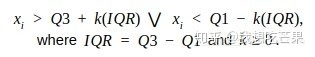
• IQR检测法往往有一个k值，一般为1.5认为$x>QU+k(IQR)||x<QL+k(IQR)$的值为异常值

Discussion

• 没有一个单一的异常检测技术是最好的
• 我们需要根据实际情况选择异常分类函数

4.7 Handling Outliers

三种常用方式处理异常值

（1）直接通过pandas的条件查询过滤

# Load library
import pandas as pd
# Create DataFrame
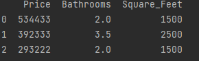
houses = pd.DataFrame()
houses['Price'] = [534433, 392333, 293222, 4322032]
houses['Bathrooms'] = [2, 3.5, 2, 116]
houses['Square_Feet'] = [1500, 2500, 1500, 48000]
# 过滤
print(houses[houses['Bathrooms'] < 20])

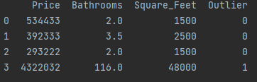
（2）方法2，通过np创建一个新的特征，这个特征通过条件判断来判别是不是Outliner

# 方法2，定义一新特征“outliner",然后使用np.where创建条件查询

# Load library
import numpy as np
# Create feature based on boolean condition
houses["Outlier"] = np.where(houses["Bathrooms"] < 20, 0, 1)
# Show data
print(houses)

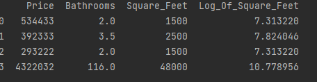
方法3：我们可以对某一特征进行数值转换来抑制他的影响

# 方法3：通过数值转换抑制某一特征异常值的影响
# Log feature
houses["Log_Of_Square_Feet"] = [np.log(x) for x in houses["Square_Feet"]]
# Show data
print(houses)

Discussion

• 处理异常值没有一尘不变的规则，需要根据具体情况来选择处理方式
• 我们如何处理异常值应该基于我们的机器学习目标。
• 如果出现异常值，要处理的话需要考虑：为什么是异常值以及最终的目标是什么？
• 不处理异常值也是一种决定
• 如果有异常值那么就不适合标准化，在这种情况下：RobustScaler是更加合理的数据归一化做法。

4.8 Discretizating Features

离散化数据

discretizatingExample.py

# Load libraries
import numpy as np
from sklearn.preprocessing import Binarizer

# Create feature
age = np.array([[6],
                [12],
                [20],
                [36],
                [65]])
# Create binarizer
binarizer = Binarizer(threshold=18)

# Transform feature
print(binarizer.fit_transform(age))

# bin feature
print(np.digitize(age, bins=[20,30,64]))

# Bin feature
print(np.digitize(age, bins=[20,30,64], right=True))

三个实例：

• binarizer:对某个阈值进行二分

• digitize可以对多个阈值进行划分

• 如果digitize的right参数为true那么只有边界右边的值才会被划分到一类种

Discussion

• 离散化对于某些问题是个非常有用的方式（原书举例了美国喝酒年龄20和21岁的差异很大的例子）
• 主要有两种方法binarizer和digitize

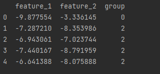
4.9 Grouping Observations Using Clustering

聚类

划分方法Kmeans

import pandas as pd
from sklearn.datasets import make_blobs
from sklearn.cluster import KMeans

features, _ = make_blobs(n_samples = 50,
                         n_features = 2,
                         centers = 3,
                         random_state = 1)

df = pd.DataFrame(features, columns=["feature_1", "feature_2"])

#  k-means 聚类
clusterer = KMeans(3, random_state=0)

# 过滤数据
clusterer.fit(features)

# 预测分类
df['group'] = clusterer.predict(features)

print(df.head(5))

Discussion

• 聚类算法将在19章中详细介绍
• k-means是一种无监督算法，最终得到一个分类的特征
• 查阅资料：K-Means(K均值聚类算法) - 知乎 (zhihu.com)
  • 即 K 均值算法，是一种常见的聚类算法。算法会将数据集分为 K 个簇，每个簇使用簇内所有样本均值来表示，将该均值称为“质心”。
  • 容易受初始质心的影响；算法简单，容易实现；算法聚类时，容易产生空簇；算法可能收敛到局部最小值。
  • 距离计算方式是 欧式距离。

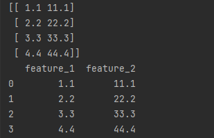
4.10 Deleteing Observations with Missing Values

删除含空值的observation

# 方法1用numpy
# Load library
import numpy as np
# Create feature matrix
features = np.array([[1.1, 11.1],
[2.2, 22.2],
[3.3, 33.3],
[4.4, 44.4],
[np.nan, 55]])
# Keep only observations that are not (denoted by ~) missing
print(features[~np.isnan(features).any(axis=1)])

# 方法2用pandas
import pandas as pd
# Load data
dataframe = pd.DataFrame(features, columns=["feature_1", "feature_2"])
# Remove observations with missing values
print(dataframe.dropna())

Discussion

• 大多数机器学习算法无法处理目标和特征数组中的任何缺失值。
• 最简单的解决方案是删除包含一个或多个缺失值的每个观察值
• 缺失数据分为三种：
  • 完全随机丢失（MCAR） 缺失值的概率与一切无关。
  • 随机失踪（MAR） 缺失值的概率不是完全随机的，而是取决于其他特征中的信息捕获
  • 非随机缺失 (MNAR) 缺失值的概率不是随机的，取决于我们的特征中未捕获的信息

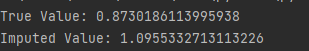
4.11 Imputing Missing Values

预测并且填充丢失的值

inputingExample.py

fancyimpute需要安装

• fancyimpute是python的第三方工具包，主要提供了各种矩阵计算、填充算法的实现。

# Load libraries
import numpy as np
from fancyimpute import KNN
from sklearn.preprocessing import StandardScaler
from sklearn.datasets import make_blobs

# Make a simulated feature matrix
features, _ = make_blobs(n_samples=1000,
                         n_features=2,
                         random_state=1)
# 标准化
scaler = StandardScaler()
standardized_features = scaler.fit_transform(features)
# 替换第一个值为NAN
true_value = standardized_features[0, 0]
standardized_features[0, 0] = np.nan
# 预测 complete已经被替换为fit_transform
features_knn_imputed = KNN(k=5, verbose=0).fit_transform(standardized_features)
# 比较
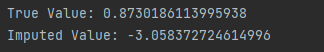
print("True Value:", true_value)
print("Imputed Value:", features_knn_imputed[0, 0])

• sklearn中的impute包的方式

#Load library
# impute已经被替代
#from sklearn.preprocessing import Imputer
from sklearn.impute import SimpleImputer

# Create SimpleImputer
mean_imputer = SimpleImputer(strategy="mean")
# Impute values
features_mean_imputed = mean_imputer.fit_transform(features)
# Compare true and imputed values
print("True Value:", true_value)
print("Imputed Value:", features_mean_imputed[0,0])

Discussion

• 替代值往往有两种主要策略。

  • 我们可以使用机器学习来预测缺失数据的值。为此，我们将具有缺失值的特征视为目标向量，并使用剩余的特征子集来预测缺失值。虽然我们可以使用广泛的机器学习算法来估算值，但流行的选择是 KNN。
  • 更具可扩展性的策略是用一些平均值填充所有缺失值。

• 两种方式各有优缺点

  • KNN 的缺点是，为了知道哪些观测值最接近缺失值，它需要计算缺失值与每个观测值之间的距离。这在较小的数据集中是合理的，但如果数据集有数百万个观测值，很快就会出现问题。
  • 均值的方式往往不像我们使用 KNN 时那样接近真实值

• fancyimpute包查询资料

  SimpleFill	用每列的平均值或中值替换缺失的条目。
  KNN	最近邻插补，它使用两行都具有观察数据的特征的均方差对样本进行加权。
  SoftImpute	通过 SVD 分解的迭代软阈值完成矩阵论文笔记 Spectral Regularization Algorithms for Learning Large IncompleteMatrices （soft-impute）_UQI-LIUWJ的博客-优快云博客
  IterativeImpute	通过以循环方式将具有缺失值的每个特征建模为其他特征的函数，来估算缺失值。类似于推荐系统笔记：使用分类模型进行协同过滤_UQI-LIUWJ的博客-优快云博客
  IterativeSVD	通过迭代低秩 SVD 分解完成矩阵。类似于 推荐系统笔记：基于SVD的协同过滤_UQI-LIUWJ的博客-优快云博客_基于svd的协同过滤
  MatrixFactorization	将不完整矩阵直接分解为低秩 U 和 V，具有每行和每列偏差以及全局偏差。
  BiScaler	行/列均值和标准差的迭代估计以获得双重归一化矩阵。 不保证收敛，但在实践中效果很好。

• KNN算法

  • (87条消息) K-近邻算法（KNN)_的博客-优快云博客_k近邻算法

  • K近邻（K-Nearest Neighbor, KNN）是一种最经典和最简单的有监督学习方法之一。

  • 原理：当对测试样本进行分类时，首先通过扫描训练样本集，找到与该测试样本最相似的个训练样本，根据这个样本的类别进行投票确定测试样本的类别。也可以通过个样本与测试样本的相似程度进行加权投票。如果需要以测试样本对应每类的概率的形式输出，可以通过个样本中不同类别的样本数量分布来进行估计。

下一章：(90条消息) Machine Learning with Python Cookbook 学习笔记 第5章_五舍橘橘的博客-优快云博客