


1. Terminologies
There are many professional terms in reinforcement learning. If you want to get started with reinforcement learning, you must understand these professional terms.
1] state and action
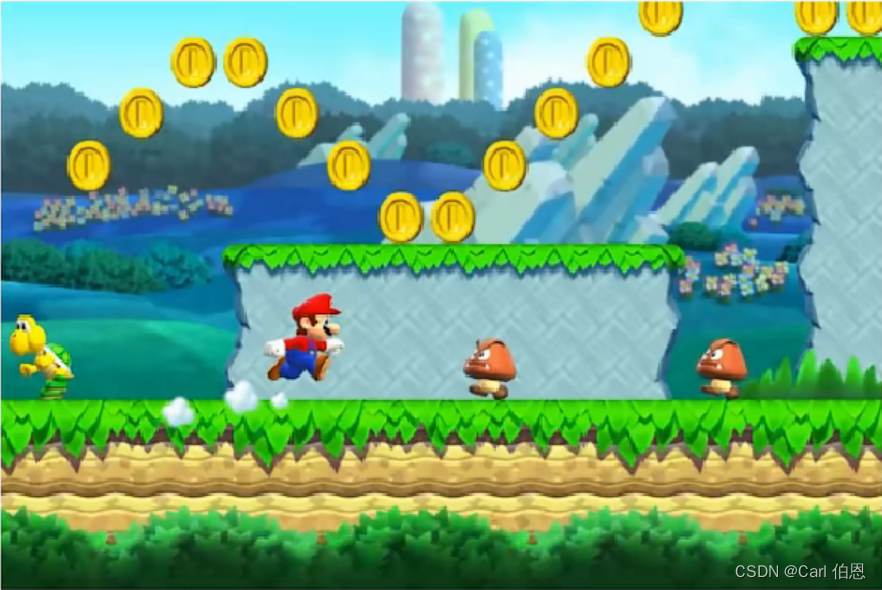
state
s
s
s (this frame)
action
a
a
a
∈
∈
∈ {left, right, up}
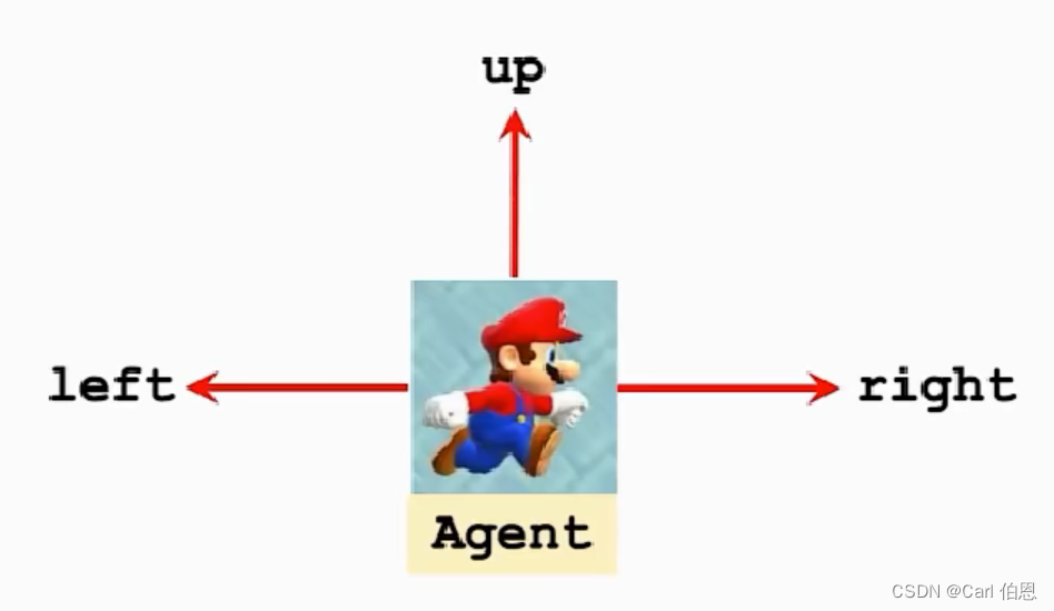
Who does the action is the agent.
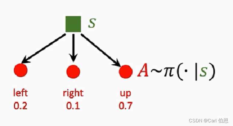
2] policy
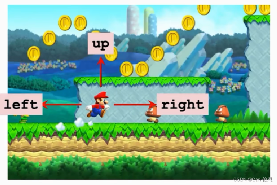
policy π \pi π : According to the observed state, make decisions and control the movement of the agent.
⋅
\cdot
⋅ Policy function
π
\pi
π :
(
s
,
a
)
(s, a)
(s,a) → [0, 1] :
π
(
a
∣
s
)
=
P
(
A
=
a
∣
S
=
s
)
.
\;\;\;\;\;\pi (a|s) = P(A=a|S=s).
π(a∣s)=P(A=a∣S=s).
⋅
\cdot
⋅It is the probability of taking action
A
=
a
A=a
A=a given
s
s
s, e.g,
⋅
π
(
l
e
f
t
∣
s
)
=
0.2
,
\;\;\;\;\;\cdot\pi (left\;|\;s) = 0.2,
⋅π(left∣s)=0.2,
⋅
π
(
r
i
g
h
t
∣
s
)
=
0.1
,
\;\;\;\;\;\cdot\pi (right|s) = 0.1,
⋅π(right∣s)=0.1,
⋅
π
(
u
p
∣
s
)
=
0.7.
\;\;\;\;\;\cdot\pi (up\;\;|\;\;s) = 0.7.
⋅π(up∣s)=0.7.
⋅
\cdot
⋅ Upon observing state
S
=
s
S = s
S=s, the agent’s action A can be random.
3] reward
reward
R
R
R
⋅
\cdot
⋅ Collect a coin:
R
R
R = +1
⋅
\cdot
⋅ Win the game:
R
R
R = +10000
⋅
\cdot
⋅ Touch a Goomba:
R
R
R = -10000
\;\;\;
(game over)
⋅
\cdot
⋅ Nothing happens:
R
R
R = +1
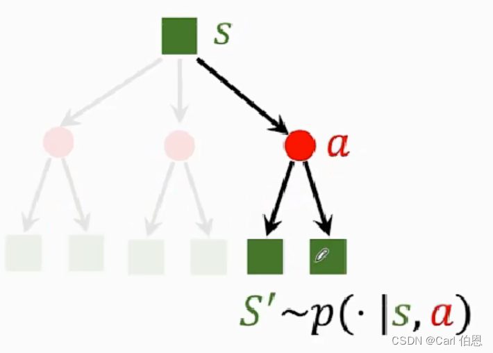
4] state transition
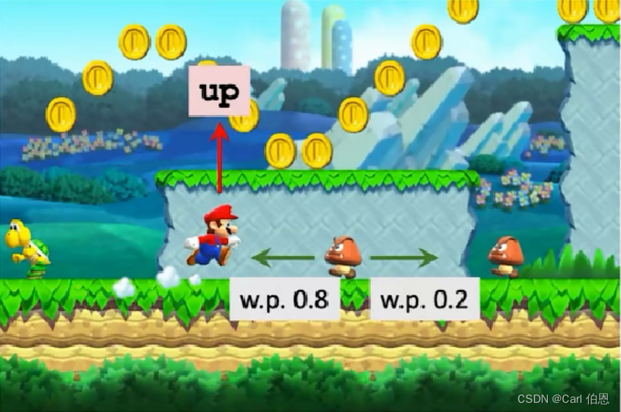
\;\;\;\;
old state
⟶
a
c
t
i
o
n
\;\;\overset{action}{\longrightarrow}\;\;
⟶actionnew state
⋅
\cdot
⋅ E.g., “up” action leads to a new state.
⋅
\cdot
⋅ State transition can be random.
⋅
\cdot
⋅ Ramdom is from the environment.
⋅
\cdot
⋅
p
(
s
′
∣
s
,
a
)
p(s^{'}|s,a)
p(s′∣s,a)=
P
(
S
′
=
s
∣
S
=
s
,
A
=
a
)
.
P(S^{'}=s|S=s,A=a).
P(S′=s∣S=s,A=a).
5] agent environment interaction
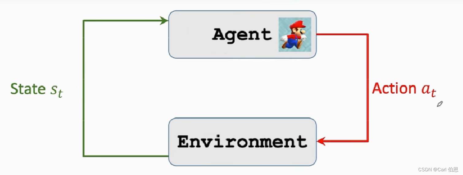
The environment here is a game program, the agent is Mary, and the state
s
t
s_{t}
st is what the environment tells us. In super Mary, we can take the current picture as the environment
s
t
s_{t}
st. when we see the state st, we need to make an action
a
t
a_{t}
at, which can be left, up, right.
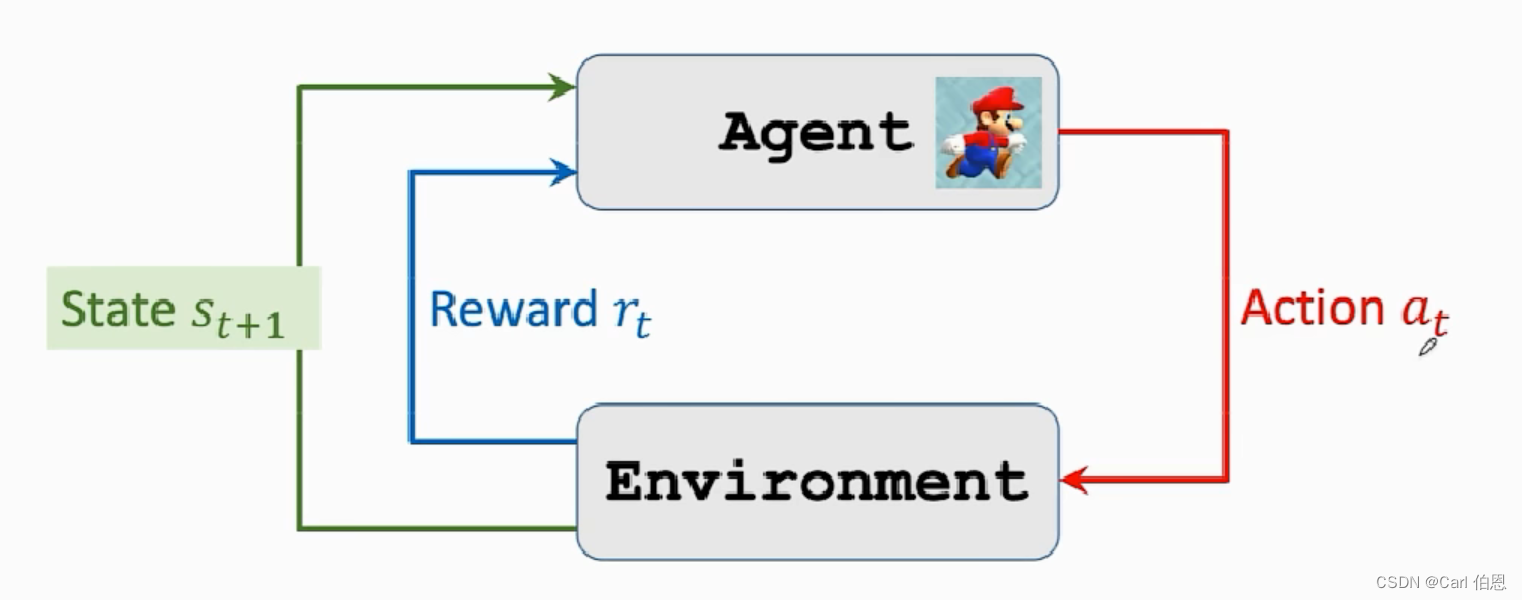
After making the action a t a_{t} at, we will get a new state and a reward r t r_{t} rt.
2. Randomness in Reinforcement Learning
1] Action have randomness
⋅
\cdot
⋅ Given state
s
s
s, the action can be random, e.g,.
\;\;\;\;
⋅
\cdot
⋅
π
(
"
l
e
f
t
∣
s
"
)
=
0.2
\pi("left|s")=0.2
π("left∣s")=0.2
\;\;\;\;
⋅
\cdot
⋅
π
(
"
r
i
g
h
t
∣
s
"
)
=
0.1
\pi("right|s")=0.1
π("right∣s")=0.1
\;\;\;\;
⋅
\cdot
⋅
π
(
"
u
p
∣
s
"
)
=
0.7
\pi("up|s")=0.7
π("up∣s")=0.7
Actions are sampled by pocily function.
2] State transitions have randomness
⋅
\cdot
⋅ Given state
S
=
s
S=s
S=s and action
A
=
a
A=a
A=a, the environment randomly generates a new state
S
′
S^{'}
S′.
The new state is sampled by the state transition function.
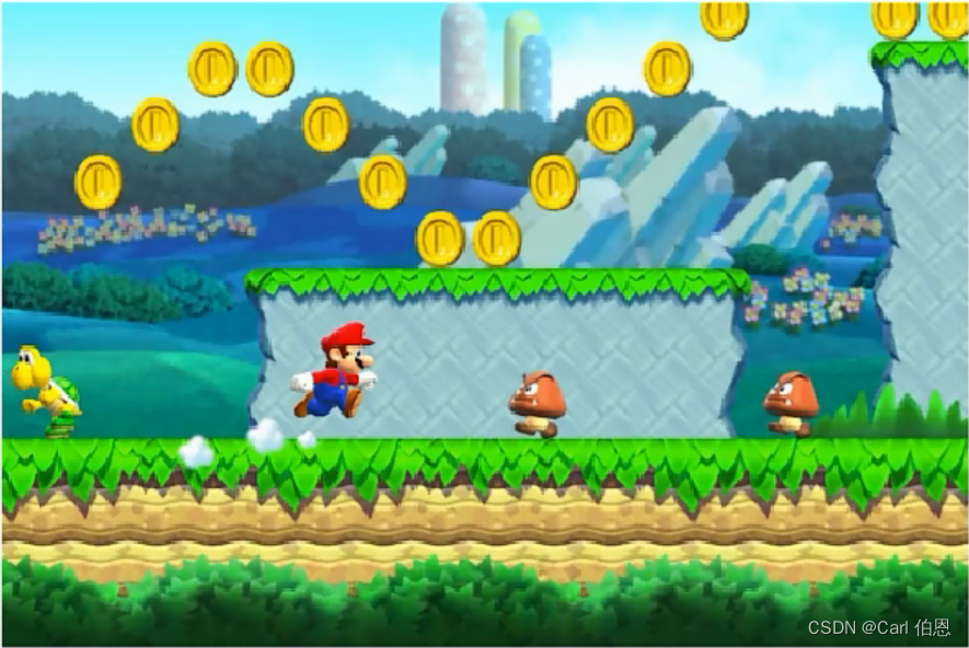
3. Play the game using AI
⋅
\cdot
⋅ Observe a frame(state
s
1
s_{1}
s1)
⋅
\cdot
⋅
⇒
\Rightarrow
⇒ Make action
a
1
a_{1}
a1 (left, right, or up)
⋅
\cdot
⋅
⇒
\Rightarrow
⇒Observe a new frame(state
s
2
s_{2}
s2) and reward
r
1
r_{1}
r1
⋅
\cdot
⋅
⇒
\Rightarrow
⇒ Make action
a
2
a_{2}
a2
⋅
\cdot
⋅
⇒
\Rightarrow
⇒ …
⋅
\cdot
⋅ (state, action, reward) trajectory:
s
1
,
a
1
,
r
1
,
s
2
,
a
2
,
r
2
,
.
.
.
.
.
.
,
s
T
,
a
T
,
r
T
.
\;\;s_{1},a_{1},r_{1},s_{2},a_{2},r_{2},......,s_{T},a_{T},r_{T}.
s1,a1,r1,s2,a2,r2,......,sT,aT,rT.
4. Rewards and Returns (important)
4.1 Rerun
Definition: Return (cumulative future reward)
⋅ \cdot ⋅ U t = R t + R t + 1 + R t + 2 + R t + 3 + . . . U_{t}=R_{t}+R_{t+1}+R_{t+2}+R_{t+3}+... Ut=Rt+Rt+1+Rt+2+Rt+3+...
Question: Are
R
t
R_{t}
Rt and
R
t
+
1
R_{t+1}
Rt+1 equally important?
⋅
\cdot
⋅ Which of the followings do you prefer?
\;\;\;
⋅
\cdot
⋅ I give you $100 right now.
\;\;\;
⋅
\cdot
⋅ I will give you $100 one year later.
⋅
\cdot
⋅ Future reward is less valuable than present reward.
⋅
\cdot
⋅
R
t
+
1
R_{t+1}
Rt+1 should be given less weight than
R
t
R_{t}
Rt
Definition: Discounted return(cumulative discounted future reward)
⋅ \cdot ⋅ γ \gamma γ: discount rate (tuning hyper-parameter).
⋅ \cdot ⋅ U t = R t + γ R t + 1 + γ 2 R t + 2 + γ 3 R t + 3 + . . . U_{t}=R_{t}+\gamma R_{t+1}+\gamma ^{2}R_{t+2}+\gamma ^{3}R_{t+3}+... Ut=Rt+γRt+1+γ2Rt+2+γ3Rt+3+...
4.2 Randomness in Returns
Definition: Discounted return(at time step t)
⋅ \cdot ⋅ U t = R t + R t + 1 + R t + 2 + R t + 3 + . . . U_{t}=R_{t}+R_{t+1}+R_{t+2}+R_{t+3}+... Ut=Rt+Rt+1+Rt+2+Rt+3+...
At time step t, the return
U
t
U_{t}
Ut is random.
⋅
\cdot
⋅ Two sources of randomness:
\;\;\;\;
1. Action can be random:
P
[
A
=
a
∣
S
=
s
]
=
π
(
a
∣
s
)
.
\;P[A=a|S=s]=\pi(a|s).
P[A=a∣S=s]=π(a∣s).
\;\;\;\;
2. New state can be random:
P
[
S
′
=
s
∣
S
=
s
,
A
=
a
]
=
p
(
s
′
∣
s
,
a
)
.
\;P[S^{'}=s|S=s,A=a]=p(s^{'}|s,a).
P[S′=s∣S=s,A=a]=p(s′∣s,a).
⋅ \cdot ⋅ For any i ≥ \geq ≥ t, the reward R i R_{i} Ri depends on S i S_{i} Si and A i A_{i} Ai.
⋅
\cdot
⋅ Thus, given
s
t
s_{t}
st, the return
U
t
U_{t}
Ut depends on the random variables:
\;\;\;
⋅
\cdot
⋅
A
t
,
A
t
+
1
,
A
t
+
2
,
.
.
.
A_{t},A_{t+1},A_{t+2},...
At,At+1,At+2,... and
S
t
+
1
,
S
t
+
2
,
.
.
.
S_{t+1},S_{t+2},...
St+1,St+2,...
5. Value Function
5.1 Action-Value Function Q ( s , a ) Q(s,a) Q(s,a)
Definition: Return (cumulative future reward)
⋅
\cdot
⋅
U
t
=
R
t
+
R
t
+
1
+
R
t
+
2
+
R
t
+
3
+
.
.
.
U_{t}=R_{t}+R_{t+1}+R_{t+2}+R_{t+3}+...
Ut=Rt+Rt+1+Rt+2+Rt+3+...
Definition: Action-value function for policy
π
\pi
π
⋅
\cdot
⋅
Q
π
(
s
t
,
a
t
)
=
E
[
U
t
∣
S
t
=
s
t
,
A
t
=
a
t
]
Q_{\pi}(s_{t},a_{t})=E[U_{t}|S_{t}=s_{t},A_{t}=a_{t}]
Qπ(st,at)=E[Ut∣St=st,At=at]
⋅ \cdot ⋅ Return U t U_{t} Ut (random variable) depends on actions A t , A t + 1 , A t + 2 , . . . A_{t},A_{t+1},A_{t+2},... At,At+1,At+2,... and S t , S t + 1 , S t + 2 , . . . S_{t},S_{t+1},S_{t+2},... St,St+1,St+2,...
⋅ \cdot ⋅ Actions are random: P [ A = a ∣ S = s ] = π ( a ∣ s ) . \;P[A=a|S=s]=\pi(a|s). P[A=a∣S=s]=π(a∣s). (Policy function)
⋅ \cdot ⋅ States are random: P [ S ′ = s ∣ S = s , A = a ] = p ( s ′ ∣ s , a ) . \;P[S^{'}=s|S=s,A=a]=p(s^{'}|s,a). P[S′=s∣S=s,A=a]=p(s′∣s,a). (State transition)
Action value function represents: if the policy function is used π \pi π, then whether it is good or bad to act a t a_{t} at in the state of s t s_{t} st, we know the policy function π \pi π, You can score all actions a a a in the current state.
Definition: Optimal action-value function
⋅
\cdot
⋅
Q
π
∗
(
s
t
,
a
t
)
=
m
a
x
π
Q_{\pi}^{*}(s_{t},a_{t})=\underset{\pi}{max}
Qπ∗(st,at)=πmax
Q
π
(
s
t
,
a
t
)
Q_{\pi}^{}(s_{t},a_{t})
Qπ(st,at)
Evaluate action
a
a
a to tell the best action.
5.2 State-Value Function V ( s ) V(s) V(s)
Definition: State-value function
⋅
\cdot
⋅
V
π
(
s
t
)
=
V_{\pi}(s_{t})=
Vπ(st)=
E
A
[
Q
π
(
s
t
,
A
)
]
=
∑
a
π
(
a
∣
s
t
)
⋅
Q
π
(
s
t
,
a
)
E_{A}[Q_{\pi}^{}(s_{t},A)]=\sum_{a} \pi(a|s_{t}) \cdot Q_{\pi}(s_{t},a)
EA[Qπ(st,A)]=∑aπ(a∣st)⋅Qπ(st,a). (Actions are discrete)
⋅ \cdot ⋅ V π ( s t ) = V_{\pi}(s_{t})= Vπ(st)= E A [ Q π ( s t , A ) ] = ∫ π ( a ∣ s t ) ⋅ Q π ( s t , a ) d a E_{A}[Q_{\pi}^{}(s_{t},A)]=\int \pi(a|s_{t}) \cdot Q_{\pi}(s_{t},a) da EA[Qπ(st,A)]=∫π(a∣st)⋅Qπ(st,a)da. (Actions are continuous)
V π ( s t ) V_{\pi}(s_{t}) Vπ(st) could make a judgment on the current situation and tell us whether we are going to win or lose, or others.
5.3 Understanding the Value Functions
⋅
\cdot
⋅ Action-value function:
Q
π
(
s
t
,
a
t
)
=
E
[
U
t
∣
S
t
=
s
t
,
A
t
=
a
t
]
Q_{\pi}(s_{t},a_{t})=E[U_{t}|S_{t}=s_{t},A_{t}=a_{t}]
Qπ(st,at)=E[Ut∣St=st,At=at].
⋅
\cdot
⋅ For policy
π
\pi
π,
Q
π
(
s
,
a
)
\;Q_{\pi} (s,a)
Qπ(s,a) evaluates how good it is for an agent to pick action
a
a
a while being in state
s
s
s.
⋅
\cdot
⋅ State-value function:
V
π
(
s
t
)
=
E
A
[
Q
π
(
s
t
,
A
)
]
V_{\pi}(s_{t})=E_{A}[Q_{\pi}^{}(s_{t},A)]
Vπ(st)=EA[Qπ(st,A)]
⋅
\cdot
⋅ For fixed policy
π
\pi
π,
V
π
(
s
)
\;V_{\pi}(s)
Vπ(s) evaluates how good the situation is in state
s
s
s.
⋅
\cdot
⋅
E
s
[
V
π
(
s
)
]
E_{s}[V_{\pi}(s)]
Es[Vπ(s)] evaluates how good the policy
π
\pi
π is.
6. How does AI control the agent?
Suppose we have a good policy
π
(
a
∣
s
)
\pi(a|s)
π(a∣s).
⋅
\cdot
⋅ Upon observe the state
s
s
,
s_{s},
ss,
⋅
\cdot
⋅ random sampling:
a
t
∽
π
(
⋅
∣
s
t
)
a_{t}\backsim\pi(\cdot|s_{t})
at∽π(⋅∣st).
Suppose we know the optimal action-value function
Q
∗
(
s
,
a
)
Q^{*}(s,a)
Q∗(s,a).
⋅
\cdot
⋅ Upon observe the state
s
t
,
s_{t},
st,
⋅
\cdot
⋅ choose the action that maximizes the values:
a
t
=
a
r
g
m
a
x
a
Q
∗
(
s
t
,
a
)
.
a_{t}=argmax_{a}Q^{*}(s_{t},a).
at=argmaxaQ∗(st,a).
7. Summary
Agent, Environment, State s s s, Action a a a, Reward r r r, Policy π ( a ∣ s ) \pi(a|s) π(a∣s), State transition p ( s ′ ∣ s , a ) p(s^{'}|s,a) p(s′∣s,a).
Return: U t = R t + γ R t + 1 + γ 2 R t + 2 + γ 3 R t + 3 + . . . U_{t}=R_{t}+\gamma R_{t+1}+\gamma ^{2}R_{t+2}+\gamma ^{3}R_{t+3}+... Ut=Rt+γRt+1+γ2Rt+2+γ3Rt+3+...
Action-value function: Q π ( s t , a t ) = E [ U t ∣ S t = s t , A t = a t ] Q_{\pi}(s_{t},a_{t})=E[U_{t}|S_{t}=s_{t},A_{t}=a_{t}] Qπ(st,at)=E[Ut∣St=st,At=at].
Optimal action-value function: Q π ∗ ( s t , a t ) = m a x π Q_{\pi}^{*}(s_{t},a_{t})=\underset {\pi}{max} Qπ∗(st,at)=πmax Q π ( s t , a t ) Q_{\pi}^{}(s_{t},a_{t}) Qπ(st,at).
State-value function: V π ( s t ) = V_{\pi}(s_{t})= Vπ(st)= E A [ Q π ( s t , A ) ] E_{A}[Q_{\pi}^{}(s_{t},A)] EA[Qπ(st,A)]


 被折叠的 条评论
为什么被折叠?
被折叠的 条评论
为什么被折叠?
 到【灌水乐园】发言


