python sklearn 实现线性回归与非线性回归_regression model python 非线性-优快云博客

本文链接：https://blog.youkuaiyun.com/weixin_49583390/article/details/120573540

该博客通过Python的sklearn库展示了如何进行线性与非线性回归分析。首先，使用线性回归模型拟合数据，然后通过多项式特征转换实现非线性回归。结果显示，非线性回归更好地拟合了带有噪声的数据。最后，给出了两种回归方程的详细表达式。

摘要生成于 C知道，由 DeepSeek-R1 满血版支持，前往体验 >

import pandas as pd
import numpy as np
import matplotlib
import random
from matplotlib import pyplot as plt
from sklearn.preprocessing import PolynomialFeatures
from sklearn.linear_model import LinearRegression

x = np.array(range(30))
temp_y = 10 + 2*x + x**2 + x**3
y = temp_y + 1500*np.random.normal(size=30)  #添加噪声

x = x.reshape(30,1)
y = y.reshape(30,1)

#线性回归
clf1 = LinearRegression()  
clf1.fit(x,y)
y_l = clf1.predict(x)  #线性回归预测值

#非线性回归
ployfeat = PolynomialFeatures(degree=3)  #根据degree的值转换为相应的多项式（非线性回归）
x_p = ployfeat.fit_transform(x)
clf2 = LinearRegression()
clf2.fit(x_p,y)

font={"family":"FangSong",'size':12}
matplotlib.rc("font",**font)
plt.figure(figsize = (12,6))
plt.plot(x,y_l,label = "线性回归")
plt.scatter(x,y,label="real value")
plt.plot(x,np.matmul(x_p,clf.coef_.reshape(4,1)) + clf.intercept_,label="非线性回归")
plt.legend()
plt.show()

print("线性回归方程为: y = {} + {}x".format(clf1.intercept_[0],clf1.coef_[0,0]))
print("非线性回归曲线方程为 y = {}+{}x+{}x^2+{}x^3".format(clf2.intercept_[0],clf2.coef_[0,1],clf2.coef_[0,2],clf2.coef_[0,3]))

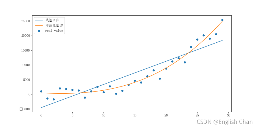
线性回归方程为: y = -4556.410727239843 + 790.8913721234021x
非线性回归曲线方程为 y = 466.91615911474946+-105.82078955667033x+12.7617011678153x^2+0.6880360959150948x^3