


基于PaddlePaddle构建ResNet18残差神经网络的食物图片分类问题
Introduction
本项目是在李宏毅机器学习课程的作业3进行的工作,任务是手动搭建一个CNN模型进行食物图片分类(11种)。
项目要求
- 请使用 CNN 搭建 model
- 不能使用额外 dataset
- 禁止使用 pre-trained model(只能自己手写CNN)
- 请不要上网寻找 label
Abstract
本文的主要内容如下:
- 1 PaddlePaddle的深度学习万能公式介绍:该
万能公式其实是进行项目研究的常规性方法步骤,本项目就是按照该步骤进行的,能够很好的作为项目开展的DEMO。 - 2 手动搭建基于标准ResNet18残差神经网络模型并改变其内部参数设置,使得提取的特征增多。最终在训练集和验证集上表现挺好,但模型存在过拟合现象,还需要进一步学习得到更好的模型。
- 3 在测试集上全部进行了预测,由于没有标签,批量展示了部分预测,预测准确率挺高的。
- 4 最后给出了简单的残差神经网络搭建的方法,通过调整模块内部Residual的数量和配置实现不同的ResNet网络。
想看预测结果直接拉到快文章末尾处……
目录
- 深度学习万能公式——PaddlePaddle
- 1 问题定义
- 2 数据准备
- 3 模型选择和开发
- 4 模型训练
- 5 模型评估和测试
- 6 模型部署
- 7 残差神经网络搭建的方法
- 8参考文献&文章&代码
- 作者介绍
- 附录
深度学习万能公式——PaddlePaddle
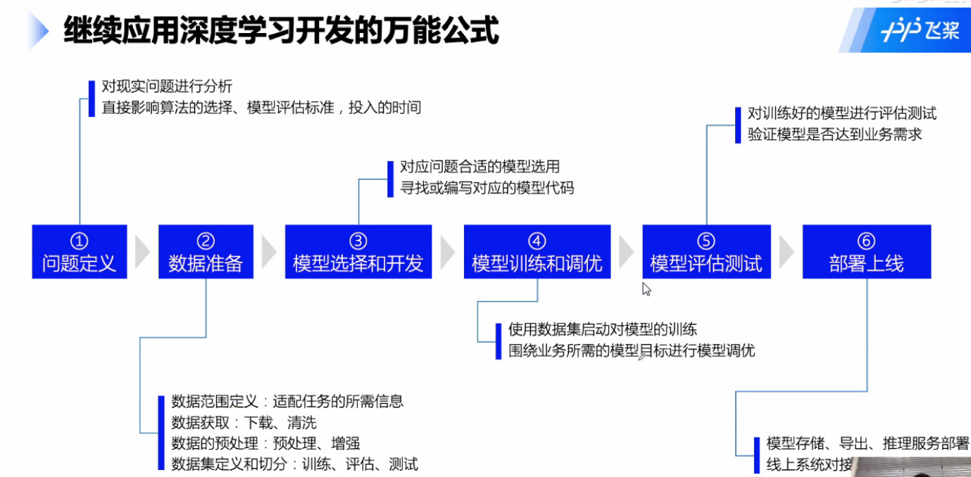
- 1 问题定义
- 2 数据准备
- 3 模型选择和开发
- 4 模型训练和调优
- 5 模型评估和测试
- 6 部署上线
1 问题定义
根据项目要求,搭建一个CNN模型实现11类食物图片的分类,属于分类问题。
2 数据准备
数据格式
下载 zip 档后解压缩会有三个资料夹,分别为training、validation 以及 testing
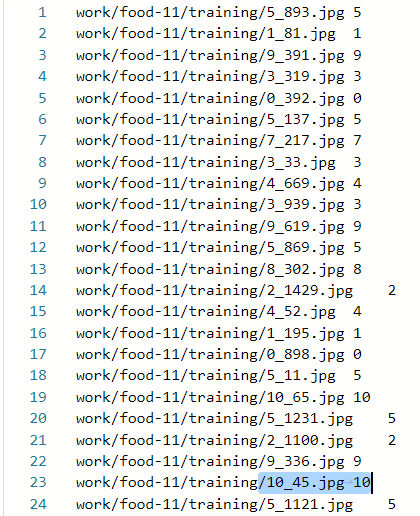
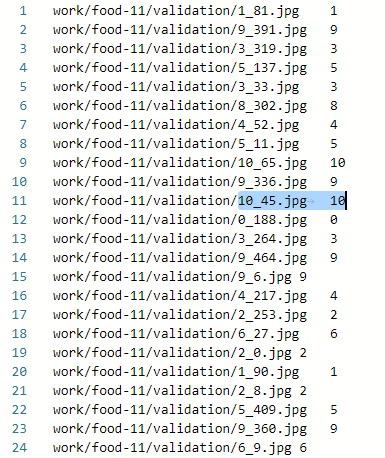
training 以及 validation 中的照片名称格式为 [类别]_[编号].jpg,例如 3_100.jpg 即为类别 3 的照片(编号不重要)
2.1 解压缩数据集
!unzip -d work data/data57075/food-11.zip # 解压缩food-11数据集
inflating: work/food-11/training/6_12.jpg
2.2 数据标注
我们先看一下解压缩后的数据集长成什么样子。
.
├── training:
│ [类别]_[编号].jpg
│ .
│ .
│ .
│
├── validation:
│ [类别]_[编号].jpg
│ .
│ .
│ .
│
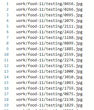
├── testing:
│ [编号].jpg
│ .
│ .
│ .
│
数据集共有三个资料夹,分别为training、validation 以及 testing。这三个文件夹里直接存放着照片,照片名称格式为 [类别]_[编号].jpg,例如 3_100.jpg 即为类别 3 的照片(编号不重要),每个文件夹里都有11类。对这些样本进行一个标注处理,最终生成train.txt/valid.txt/test.txt三个数据标注文件。
import io
import os
from PIL import Image
from config import get  # 配置函数文件包括了多种参数的设置,详细代码见附录
# 数据集根目录
DATA_ROOT = 'work/food-11'

# 标注生成函数
def generate_annotation(mode):
    # 建立标注文件
    with open('{}/{}.txt'.format(DATA_ROOT, mode), 'w') as f:
        # 对应每个用途的数据文件夹,train/valid/test
        train_dir = '{}/{}'.format(DATA_ROOT, mode)
        # train_dir = work/food-11/training

        # 图像样本所在的路径
        image_path = '{}'.format(train_dir)

        # image_path = #'work/food-11/training'

        # 遍历所有图像
        for image in os.listdir(image_path):
            # 图像完整路径和名称
            image_file = '{}/{}'.format(image_path, image)
            for k in image:
                if k=='_':   # 如果图片名称有下划线‘—’
                    stop = image.index(k)   # 下划线所在索引
                    label_index = image[0:stop] # image的索引从0——下划线前的数字为为图片的标签
                    label_index =int(label_index)
            try:
                # 验证图片格式是否ok
                with open(image_file, 'rb') as f_img:
                    image = Image.open(io.BytesIO(f_img.read()))
                    image.load()

                    if image.mode == 'RGB':
                        f.write('{}\t{}\n'.format(image_file, label_index))
            except:
                continue

generate_annotation('training')  # 生成训练集标注文件
generate_annotation('validation')  # 生成验证集标注文件
训练集和验证集标注文件
由于测试数据集没有标签,所以只生成其数据集的路径文件
# 数据集根目录
DATA_ROOT = 'work/food-11'

def generate_annotation(mode):

    with open('{}/{}.txt'.format(DATA_ROOT, mode), 'w') as f:
        # 对应每个用途的数据文件夹,train/valid/test
        train_dir = '{}/{}'.format(DATA_ROOT, mode)
        # train_dir = work/food-11/training

        # 图像样本所在的路径
        image_path = '{}'.format(train_dir)
        # image_path = #'work/food-11/training'
        # 遍历所有图像
        for image in os.listdir(image_path):
            # 图像完整路径和名称
            image_file = '{}/{}'.format(image_path, image)
            try:
                # 验证图片格式是否ok
                with open(image_file, 'rb') as f_img:
                    image = Image.open(io.BytesIO(f_img.read()))
                    image.load()

                    if image.mode == 'RGB':
                        f.write('{}\n'.format(image_file))
            except:
                continue
 # 生成测试集
generate_annotation('testing')
测试集路径文件
2.3 数据集定义
接下来我们使用标注好的文件进行数据集类的定义,方便后续模型训练使用。
2.3.1 导入相关库
import paddle
import numpy as np
from config import get
print(paddle.__version__)
2.0.1
我们数据集的代码实现是在dataset.py中。
# data.py 文件包括了图片数据的预处理,详细代码见附录
from dataset import ZodiacDataset
2.3.2 实例化数据集类
根据所使用的数据集需求实例化数据集类,并查看总样本量。
training_dataset = ZodiacDataset(mode='training')
validation_dataset = ZodiacDataset(mode='validation')
print('训练数据集:{}张; 验证数据集:{}张'.format(len(training_dataset),len(validation_dataset)))
训练数据集:9866张; 验证数据集:3430张
2.3.3 数据集查看
print('图片:')
print(type(training_dataset[1][0]))
print(training_dataset[1][0])
print('标签:')
print(type(training_dataset[1][1]))
print(training_dataset[1][1])
图片:
<class 'paddle.VarBase'>
Tensor(shape=[3, 224, 224], dtype=float32, place=CPUPlace, stop_gradient=True,
       [[[-2.11790395, -2.11790395, -2.11790395, ..., -2.11790395, -2.11790395, -2.11790395],
         [-2.11790395, -2.11790395, -2.11790395, ..., -2.11790395, -2.11790395, -2.11790395],
         [-2.11790395, -2.11790395, -2.11790395, ..., -2.11790395, -2.11790395, -2.11790395],
         ...,
         [-2.11790395, -2.11790395, -2.11790395, ..., -2.11790395, -2.11790395, -2.11790395],
         [-2.11790395, -2.11790395, -2.11790395, ..., -2.11790395, -2.11790395, -2.11790395],
         [-2.11790395, -2.11790395, -2.11790395, ..., -2.11790395, -2.11790395, -2.11790395]],

        [[-2.03571415, -2.03571415, -2.03571415, ..., -2.03571415, -2.03571415, -2.03571415],
         [-2.03571415, -2.03571415, -2.03571415, ..., -2.03571415, -2.03571415, -2.03571415],
         [-2.03571415, -2.03571415, -2.03571415, ..., -2.03571415, -2.03571415, -2.03571415],
         ...,
         [-2.03571415, -2.03571415, -2.03571415, ..., -2.03571415, -2.03571415, -2.03571415],
         [-2.03571415, -2.03571415, -2.03571415, ..., -2.03571415, -2.03571415, -2.03571415],
         [-2.03571415, -2.03571415, -2.03571415, ..., -2.03571415, -2.03571415, -2.03571415]],

        [[-1.80444443, -1.80444443, -1.80444443, ..., -1.80444443, -1.80444443, -1.80444443],
         [-1.80444443, -1.80444443, -1.80444443, ..., -1.80444443, -1.80444443, -1.80444443],
         [-1.80444443, -1.80444443, -1.80444443, ..., -1.80444443, -1.80444443, -1.80444443],
         ...,
         [-1.80444443, -1.80444443, -1.80444443, ..., -1.80444443, -1.80444443, -1.80444443],
         [-1.80444443, -1.80444443, -1.80444443, ..., -1.80444443, -1.80444443, -1.80444443],
         [-1.80444443, -1.80444443, -1.80444443, ..., -1.80444443, -1.80444443, -1.80444443]]])
标签:
<class 'numpy.ndarray'>
1
3 模型选择和开发
根据题目要求使用 CNN 搭建 model并且禁止使用 pre-trained model(只能自己手写CNN)。值得一提的是,模型组网一般共有三组方法,以PaddlePaddle框架为例:
- (1)Sequential 组网
顺序容器。子Layer将按构造函数参数的顺序添加到此容器中。传递给构造函数的参数可以Layers或可迭代的name Layer元组。 - (2)SubClass 组网
针对一些比较复杂的网络结构,就可以使用Layer子类定义的方式来进行模型代码编写,在__init__构造函数中进行组网Layer的声明,在forward中使用声明的Layer变量进行前向计算。 - (3)飞桨框架内置模型
飞桨框架内置的模型,路径为 paddle.vision.models。那么根据要求,只能使用前两种方法来搭建模型
3.1 网络构建
由与本次分类的类别较多,训练的数据为分辨率较大的彩色图片,因此选择SubClass 组网方法来搭建Resnet18网络来完成分类任务。
3.1.1深度残差网络介绍
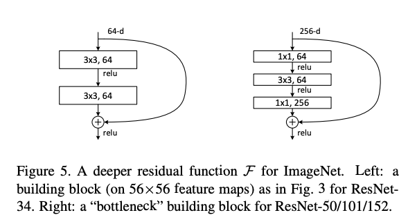
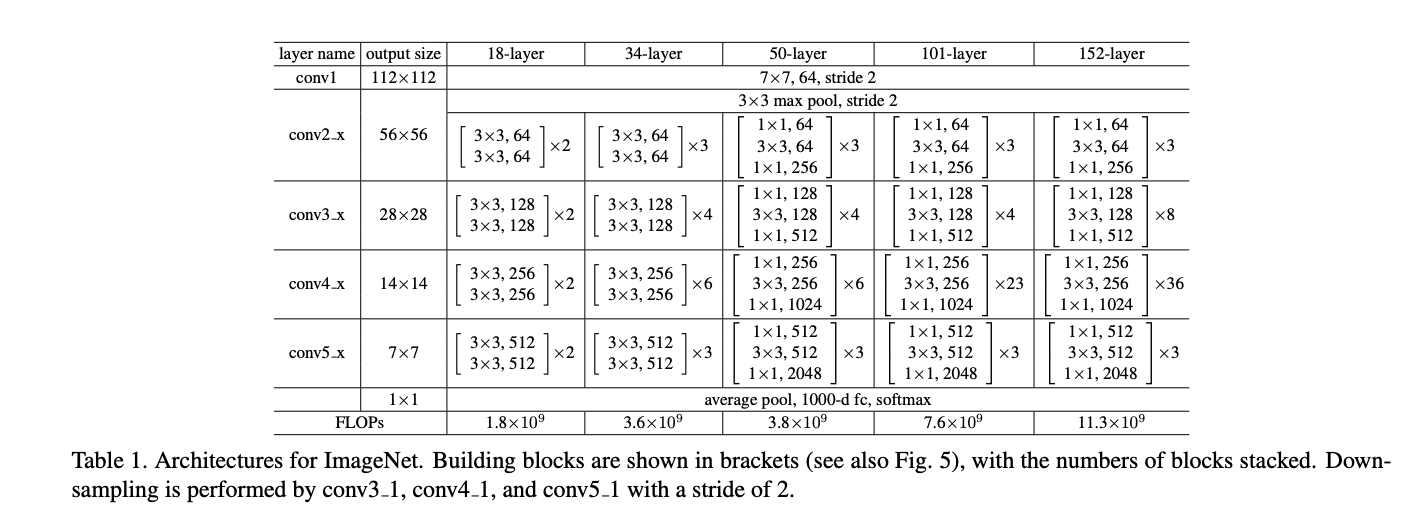
2015 年,微软亚洲研究院何恺明等人发表了基于 Skip Connection 的深度残差网络(Residual Neural Network,简称 ResNet)算法,并提出了18层、34 层、50层、101层、152层的 ResNet-18、ResNet-34、ResNet-50、ResNet-101 和 ResNet-152 等模型,如表1所示,甚至成功训练出层数达到 1202 层的极深层神经网络。ResNet 在 ILSVRC 2015挑战赛ImageNet数据集上的分类、检测等任务上面均获得了最好性能,ResNet 论文至今已经获得超 25000的引用量,可见 ResNet 在人工智能行业的影响力。ResNet 通过在卷积层的输入和输出之间添加 Skip Connection 实现层数回退机制,如下图1所示,输入𝒙通过两个卷积层,得到特征变换后的输出ℱ(𝒙),与输入𝒙进行对应元素的相加运算,得到最终输出ℋ(𝒙):
ℋ(𝒙) = 𝒙 + ℱ(𝒙)
ℋ(𝒙)叫作残差模块(Residual Block,简称 ResBlock)。由于被 Skip Connection 包围的卷积神经网络需要学习映射ℱ(𝒙) = ℋ(𝒙) − 𝒙,故称为残差网络 。
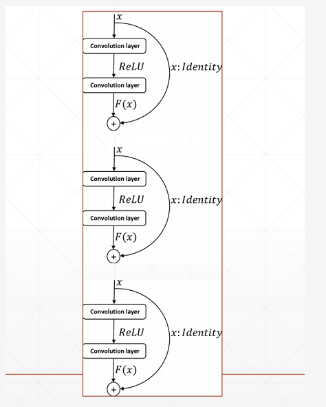
Res Block:深度残差网络通过堆叠残差模块,达到了较深的网络层数,从而获得了训练稳定、性能优越的深层网络模型,如图2所示。
1)残差区块
2) Res Block
3)ResNet系列网络
4)ResNet其他版本
3.1.2 ResNet18
标准的 ResNet18 接受输入为3x224x224大小的图片数据。 ResNet18 网络结构如下图所示。
ResNet18网络结构
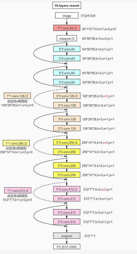
在设计深度卷积神经网络时,一般按照特征图高宽ℎ/𝑤逐渐减少,通道数𝑐逐渐增大的经验法则。可以通过堆叠通道数逐渐增大的 Res Block 来实现高层特征的提取,
3.1.3 ResNet18模型
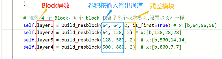
通过调整每个 Res Block 的堆叠数量和通道数可以产生不同的 ResNet,如通过 64-64-128-128-256-256-512-512 通道数配置,共8个Res Block,可得到 ResNet18 的网络模型。每个ResBlock 包含了 2 个主要的卷积层,因此卷积层数量是8x2 = 16,加上网络首末尾的全连接层,共 18 层。创建 ResNet18实现如下:
在设计深度卷积神经网络时,一般按照特征图高宽ℎ/𝑤逐渐减少,通道数𝑐逐渐增大的经验法则。可以通过堆叠通道数逐渐增大的Res Block来实现高层特征的提取,通过build_resblock可以一次完成多个残差模块的新建。代码如下:
注:
由于本次分类任务难度较大,数据集数据较少,输入的图片为3通道,因此标准的resnet18网络还算比较简单。主要在于其最终提取的特征为512个(由设置的通道数决定64-64-128-128-256-256-512-512 通道数配置),这是相对较少的。
针对上述标准resnet18存在提取特征较少的问题,我在resnet18网络基础上,对通道数目进行了设置,使得最终提取的特征为720个(64-64-150-150-360-360-720-720),网络的参数也随之增多。
import paddle
import paddle.nn as nn
import paddle.nn.functional as F

# 首先实现中间两个卷积层,Skip Connection 1x1 卷积层的残差模块。代码如下:
# 残差模块
class Residual(nn.Layer):
    def __init__(self, in_channel, out_channel, use_conv1x1=False, stride=1):
        super(Residual, self).__init__()

        # 第一个卷积单元
        self.conv1 = nn.Conv2D(in_channel, out_channel, kernel_size=3, padding=1, stride=stride)
        self.bn1 = nn.BatchNorm2D(out_channel)
        self.relu = nn.ReLU()

        # 第二个卷积单元
        self.conv2 = nn.Conv2D(out_channel, out_channel, kernel_size=3, padding=1)
        self.bn2 = nn.BatchNorm2D(out_channel)

        if use_conv1x1: #使用1x1卷积核完成shape匹配,stride=2实现下采样
            self.skip = nn.Conv2D(in_channel, out_channel, kernel_size=1, stride=stride)
        else:
            self.skip = None


    def forward(self, x):
        # 前向计算
        # [b, c, h, w], 通过第一个卷积单元
        out = self.conv1(x)
        out = self.bn1(out)
        out = self.relu(out)
        # 通过第二个卷积单元
        out = self.conv2(out)
        out = self.bn2(out)
        #  通过 identity 模块
        if self.skip:
            x = self.skip(x)
        #  2 条路径输出直接相加,然后输入激活函数
        output = F.relu(out + x)

        return output
# 通过build_resblock 可以一次完成2个残差模块的创建。代码如下:
def build_resblock(in_channel, out_channel, num_layers, is_first=False):
    if is_first:
        assert in_channel == out_channel
    block_list = []
    for i in range(num_layers):
        if i == 0 and not is_first:
            block_list.append(Residual(in_channel, out_channel, use_conv1x1=True, stride=2))
        else:
            block_list.append(Residual(out_channel, out_channel))
    resNetBlock = nn.Sequential(*block_list) #用*号可以把list列表展开为元素
    return resNetBlock

# 下面来实现ResNet18网络模型。代码如下:
class ResNet18_1(nn.Layer):
    # 继承paddle.nn.Layer定义网络结构
    def __init__(self,num_classes=11):
        super(ResNet18_1, self).__init__()
        # 初始化函数(根网络,预处理)
        # x:[b, c, h ,w]=[b,3,224,224]
        self.features = nn.Sequential(
            nn.Conv2D(in_channels=3, out_channels=64, kernel_size=7,
            stride=2, padding=3),# 第一层卷积,x:[b,64,112,112]
            nn.BatchNorm2D(64),# 归一化层
            nn.ReLU(),
            nn.MaxPool2D(kernel_size=3, stride=2, padding=1)# 最大池化,下采样,x:[b,64,56,56]
        )

        # 堆叠 4 个 Block,每个 block 包含了多个残差模块,设置步长不一样
        self.layer1 = build_resblock(64, 64, 2, is_first=True) # x:[b,64,56,56]
        self.layer2 = build_resblock(64, 150, 2) # x:[b,150,28,28]
        self.layer3 = build_resblock(150, 360, 2)  # x:[b,360,14,14]
        self.layer4 = build_resblock(360, 720, 2)  # x:[b,720,7,7]

        # 通过 Pooling 层将高宽降低为 1x1,[b,720,1,1]
        self.avgpool = nn.AdaptiveAvgPool2D(1)
        # 需要拉平为[b,720],不能直接输出连接线性层
        self.flatten = nn.Flatten()
        # 最后连接一个全连接层分类
        self.fc = nn.Linear(in_features=720,out_features=num_classes)

    def forward(self, inputs):
        # 前向计算函数:通过根网络
        x = self.features(inputs)
        # 一次通过 4 个模块
        x = self.layer1(x)
        x = self.layer2(x)
        x = self.layer3(x)
        x = self.layer4(x)
        # 通过池化层
        x = self.avgpool(x)
        # 拉平
        x = self.flatten(x)
        # 通过全连接层
        x = self.fc(x)

        return x
3.1.4 可视化模型
模型的总参数如下:比标准的ResNet18网络参数多了一千万左右。
Total params: 21,523,725
Trainable params: 21,502,765
Non-trainable params: 20,960
# ResNet18网络
model = ResNet18_1()
# 可视化模型
paddle.summary(model,(-1,3,224,224))
-------------------------------------------------------------------------------
   Layer (type)         Input Shape          Output Shape         Param #
===============================================================================
     Conv2D-1        [[1, 3, 224, 224]]   [1, 64, 112, 112]        9,472
   BatchNorm2D-1    [[1, 64, 112, 112]]   [1, 64, 112, 112]         256
      ReLU-1        [[1, 64, 112, 112]]   [1, 64, 112, 112]          0
    MaxPool2D-1     [[1, 64, 112, 112]]    [1, 64, 56, 56]           0
     Conv2D-2        [[1, 64, 56, 56]]     [1, 64, 56, 56]        36,928
   BatchNorm2D-2     [[1, 64, 56, 56]]     [1, 64, 56, 56]          256
      ReLU-2         [[1, 64, 56, 56]]     [1, 64, 56, 56]           0
     Conv2D-3        [[1, 64, 56, 56]]     [1, 64, 56, 56]        36,928
   BatchNorm2D-3     [[1, 64, 56, 56]]     [1, 64, 56, 56]          256
    Residual-1       [[1, 64, 56, 56]]     [1, 64, 56, 56]           0
     Conv2D-4        [[1, 64, 56, 56]]     [1, 64, 56, 56]        36,928
   BatchNorm2D-4     [[1, 64, 56, 56]]     [1, 64, 56, 56]          256
      ReLU-3         [[1, 64, 56, 56]]     [1, 64, 56, 56]           0
     Conv2D-5        [[1, 64, 56, 56]]     [1, 64, 56, 56]        36,928
   BatchNorm2D-5     [[1, 64, 56, 56]]     [1, 64, 56, 56]          256
    Residual-2       [[1, 64, 56, 56]]     [1, 64, 56, 56]           0
     Conv2D-6        [[1, 64, 56, 56]]     [1, 150, 28, 28]       86,550
   BatchNorm2D-6     [[1, 150, 28, 28]]    [1, 150, 28, 28]         600
      ReLU-4         [[1, 150, 28, 28]]    [1, 150, 28, 28]          0
     Conv2D-7        [[1, 150, 28, 28]]    [1, 150, 28, 28]       202,650
   BatchNorm2D-7     [[1, 150, 28, 28]]    [1, 150, 28, 28]         600
     Conv2D-8        [[1, 64, 56, 56]]     [1, 150, 28, 28]        9,750
    Residual-3       [[1, 64, 56, 56]]     [1, 150, 28, 28]          0
     Conv2D-9        [[1, 150, 28, 28]]    [1, 150, 28, 28]       202,650
   BatchNorm2D-8     [[1, 150, 28, 28]]    [1, 150, 28, 28]         600
      ReLU-5         [[1, 150, 28, 28]]    [1, 150, 28, 28]          0
     Conv2D-10       [[1, 150, 28, 28]]    [1, 150, 28, 28]       202,650
   BatchNorm2D-9     [[1, 150, 28, 28]]    [1, 150, 28, 28]         600
    Residual-4       [[1, 150, 28, 28]]    [1, 150, 28, 28]          0
     Conv2D-11       [[1, 150, 28, 28]]    [1, 360, 14, 14]       486,360
  BatchNorm2D-10     [[1, 360, 14, 14]]    [1, 360, 14, 14]        1,440
      ReLU-6         [[1, 360, 14, 14]]    [1, 360, 14, 14]          0
     Conv2D-12       [[1, 360, 14, 14]]    [1, 360, 14, 14]      1,166,760
  BatchNorm2D-11     [[1, 360, 14, 14]]    [1, 360, 14, 14]        1,440
     Conv2D-13       [[1, 150, 28, 28]]    [1, 360, 14, 14]       54,360
    Residual-5       [[1, 150, 28, 28]]    [1, 360, 14, 14]          0
     Conv2D-14       [[1, 360, 14, 14]]    [1, 360, 14, 14]      1,166,760
  BatchNorm2D-12     [[1, 360, 14, 14]]    [1, 360, 14, 14]        1,440
      ReLU-7         [[1, 360, 14, 14]]    [1, 360, 14, 14]          0
     Conv2D-15       [[1, 360, 14, 14]]    [1, 360, 14, 14]      1,166,760
  BatchNorm2D-13     [[1, 360, 14, 14]]    [1, 360, 14, 14]        1,440
    Residual-6       [[1, 360, 14, 14]]    [1, 360, 14, 14]          0
     Conv2D-16       [[1, 360, 14, 14]]     [1, 720, 7, 7]       2,333,520
  BatchNorm2D-14      [[1, 720, 7, 7]]      [1, 720, 7, 7]         2,880
      ReLU-8          [[1, 720, 7, 7]]      [1, 720, 7, 7]           0
     Conv2D-17        [[1, 720, 7, 7]]      [1, 720, 7, 7]       4,666,320
  BatchNorm2D-15      [[1, 720, 7, 7]]      [1, 720, 7, 7]         2,880
     Conv2D-18       [[1, 360, 14, 14]]     [1, 720, 7, 7]        259,920
    Residual-7       [[1, 360, 14, 14]]     [1, 720, 7, 7]           0
     Conv2D-19        [[1, 720, 7, 7]]      [1, 720, 7, 7]       4,666,320
  BatchNorm2D-16      [[1, 720, 7, 7]]      [1, 720, 7, 7]         2,880
      ReLU-9          [[1, 720, 7, 7]]      [1, 720, 7, 7]           0
     Conv2D-20        [[1, 720, 7, 7]]      [1, 720, 7, 7]       4,666,320
  BatchNorm2D-17      [[1, 720, 7, 7]]      [1, 720, 7, 7]         2,880
    Residual-8        [[1, 720, 7, 7]]      [1, 720, 7, 7]           0
AdaptiveAvgPool2D-1   [[1, 720, 7, 7]]      [1, 720, 1, 1]           0
     Flatten-1        [[1, 720, 1, 1]]         [1, 720]              0
     Linear-1            [[1, 720]]            [1, 11]             7,931
===============================================================================
Total params: 21,523,725
Trainable params: 21,502,765
Non-trainable params: 20,960
-------------------------------------------------------------------------------
Input size (MB): 0.57
Forward/backward pass size (MB): 60.45
Params size (MB): 82.11
Estimated Total Size (MB): 143.13
-------------------------------------------------------------------------------
{'total_params': 21523725, 'trainable_params': 21502765}
# 封装模型
model_1 = paddle.Model(model)
4 模型训练
4.1 模型配置与训练
- 优化器:Momentum
- 损失函数:交叉熵(cross entropy)
- 评估指标:Accuracy
# get()函数的超参数在文件config.py文件里设置

EPOCHS = get('epochs') #50
BATCH_SIZE = get('batch_size') # 128

# 设置学习率
def create_optim(parameters):
    step_each_epoch = get('total_images') // get('batch_size')
    lr = paddle.optimizer.lr.CosineAnnealingDecay(learning_rate=get('LEARNING_RATE.params.lr'),
                                                  T_max=step_each_epoch * EPOCHS)

    return paddle.optimizer.Momentum(learning_rate=lr,
                                     parameters=parameters,
                                     weight_decay=paddle.regularizer.L2Decay(get('OPTIMIZER.regularizer.factor')))

# 模型训练配置
model_1.prepare(create_optim(model.parameters()),  # 优化器
              paddle.nn.CrossEntropyLoss(),        # 损失函数
              paddle.metric.Accuracy()) # 评估指标

# 训练可视化VisualDL工具的回调函数
visualdl = paddle.callbacks.VisualDL(log_dir='visualdl_log')
# 启动模型全流程训练
model_1.fit(training_dataset,         # 训练数据集
          validation_dataset,       # 评估数据集
          epochs=EPOCHS,            # 总的训练轮次
          batch_size=BATCH_SIZE,    # 批次计算的样本量大小
          shuffle=True,             # 是否打乱样本集
          verbose=1,                # 日志展示格式
          save_dir='./chk_points1/', # 分阶段的训练模型存储路径
          save_freq=25,             # 保存模型的频率
          callbacks=[visualdl])     # 回调函数使用
The loss value printed in the log is the current step, and the metric is the average value of previous step.
Epoch 1/50
/opt/conda/envs/python35-paddle120-env/lib/python3.7/site-packages/paddle/fluid/layers/utils.py:77: DeprecationWarning: Using or importing the ABCs from 'collections' instead of from 'collections.abc' is deprecated, and in 3.8 it will stop working
  return (isinstance(seq, collections.Sequence) and
/opt/conda/envs/python35-paddle120-env/lib/python3.7/site-packages/paddle/nn/layer/norm.py:648: UserWarning: When training, we now always track global mean and variance.
  "When training, we now always track global mean and variance.")

step 78/78 [==============================] - loss: 2.3041 - acc: 0.2836 - 1s/step
save checkpoint at /home/aistudio/chk_points1/0
Eval begin...
The loss value printed in the log is the current batch, and the metric is the average value of previous step.
step 27/27 [==============================] - loss: 2.1855 - acc: 0.2341 - 1s/step
Eval samples: 3430
Epoch 2/50
step 78/78 [==============================] - loss: 2.0412 - acc: 0.3904 - 1s/step
Eval begin...
The loss value printed in the log is the current batch, and the metric is the average value of previous step.
step 27/27 [==============================] - loss: 1.6591 - acc: 0.3799 - 1s/step
Eval samples: 3430
Epoch 3/50
step 78/78 [==============================] - loss: 1.8930 - acc: 0.4360 - 1s/step
Eval begin...
The loss value printed in the log is the current batch, and the metric is the average value of previous step.
step 27/27 [==============================] - loss: 1.5796 - acc: 0.4233 - 1s/step
Eval samples: 3430
Epoch 4/50
step 78/78 [==============================] - loss: 1.9797 - acc: 0.4654 - 1s/step
Eval begin...
The loss value printed in the log is the current batch, and the metric is the average value of previous step.
step 27/27 [==============================] - loss: 1.5597 - acc: 0.4187 - 1s/step
Eval samples: 3430
Epoch 5/50
step 78/78 [==============================] - loss: 2.0698 - acc: 0.4897 - 1s/step
Eval begin...
The loss value printed in the log is the current batch, and the metric is the average value of previous step.
step 27/27 [==============================] - loss: 1.4181 - acc: 0.4566 - 1s/step
Eval samples: 3430
Epoch 6/50
step 78/78 [==============================] - loss: 1.6114 - acc: 0.5084 - 1s/step
Eval begin...
The loss value printed in the log is the current batch, and the metric is the average value of previous step.
step 27/27 [==============================] - loss: 1.3376 - acc: 0.4837 - 1s/step
Eval samples: 3430
Epoch 7/50
step 78/78 [==============================] - loss: 1.7975 - acc: 0.5249 - 1s/step
Eval begin...
The loss value printed in the log is the current batch, and the metric is the average value of previous step.
step 27/27 [==============================] - loss: 1.8178 - acc: 0.4029 - 1s/step
Eval samples: 3430
Epoch 8/50
step 78/78 [==============================] - loss: 1.4649 - acc: 0.5424 - 1s/step
Eval begin...
The loss value printed in the log is the current batch, and the metric is the average value of previous step.
step 27/27 [==============================] - loss: 1.3349 - acc: 0.4834 - 1s/step
Eval samples: 3430
Epoch 9/50
step 78/78 [==============================] - loss: 0.9464 - acc: 0.5576 - 1s/step
Eval begin...
The loss value printed in the log is the current batch, and the metric is the average value of previous step.
step 27/27 [==============================] - loss: 1.1288 - acc: 0.5274 - 1s/step
Eval samples: 3430
Epoch 10/50
step 78/78 [==============================] - loss: 1.0115 - acc: 0.5783 - 1s/step
Eval begin...
The loss value printed in the log is the current batch, and the metric is the average value of previous step.
step 27/27 [==============================] - loss: 1.2323 - acc: 0.5341 - 1s/step
Eval samples: 3430
Epoch 11/50
step 78/78 [==============================] - loss: 1.6468 - acc: 0.5853 - 1s/step
Eval begin...
The loss value printed in the log is the current batch, and the metric is the average value of previous step.
step 27/27 [==============================] - loss: 1.4320 - acc: 0.4921 - 1s/step
Eval samples: 3430
Epoch 12/50
step 78/78 [==============================] - loss: 0.9343 - acc: 0.5934 - 1s/step
Eval begin...
The loss value printed in the log is the current batch, and the metric is the average value of previous step.
step 27/27 [==============================] - loss: 1.0640 - acc: 0.5475 - 1s/step
Eval samples: 3430
Epoch 13/50
step 78/78 [==============================] - loss: 0.7966 - acc: 0.6022 - 1s/step
Eval begin...
The loss value printed in the log is the current batch, and the metric is the average value of previous step.
step 27/27 [==============================] - loss: 1.1968 - acc: 0.5213 - 1s/step
Eval samples: 3430
Epoch 14/50
step 78/78 [==============================] - loss: 1.1216 - acc: 0.6035 - 1s/step
Eval begin...
The loss value printed in the log is the current batch, and the metric is the average value of previous step.
step 27/27 [==============================] - loss: 1.0251 - acc: 0.5563 - 1s/step
Eval samples: 3430
Epoch 15/50
step 78/78 [==============================] - loss: 0.9137 - acc: 0.6237 - 1s/step
Eval begin...
The loss value printed in the log is the current batch, and the metric is the average value of previous step.
step 27/27 [==============================] - loss: 1.0920 - acc: 0.5950 - 1s/step
Eval samples: 3430
Epoch 16/50
step 78/78 [==============================] - loss: 1.6122 - acc: 0.6239 - 1s/step
Eval begin...
The loss value printed in the log is the current batch, and the metric is the average value of previous step.
step 27/27 [==============================] - loss: 1.0231 - acc: 0.5816 - 1s/step
Eval samples: 3430
Epoch 17/50
step 78/78 [==============================] - loss: 0.9047 - acc: 0.6354 - 1s/step
Eval begin...
The loss value printed in the log is the current batch, and the metric is the average value of previous step.
step 27/27 [==============================] - loss: 1.0294 - acc: 0.5723 - 1s/step
Eval samples: 3430
Epoch 18/50
step 78/78 [==============================] - loss: 1.4858 - acc: 0.6421 - 1s/step
Eval begin...
The loss value printed in the log is the current batch, and the metric is the average value of previous step.
step 27/27 [==============================] - loss: 0.9666 - acc: 0.6017 - 1s/step
Eval samples: 3430
Epoch 19/50
step 78/78 [==============================] - loss: 1.0395 - acc: 0.6494 - 1s/step
Eval begin...
The loss value printed in the log is the current batch, and the metric is the average value of previous step.
step 27/27 [==============================] - loss: 1.0967 - acc: 0.5341 - 1s/step
Eval samples: 3430
Epoch 20/50
step 78/78 [==============================] - loss: 1.6718 - acc: 0.6713 - 1s/step
Eval begin...
The loss value printed in the log is the current batch, and the metric is the average value of previous step.
step 27/27 [==============================] - loss: 0.8613 - acc: 0.6265 - 1s/step
Eval samples: 3430
Epoch 21/50
step 78/78 [==============================] - loss: 1.2523 - acc: 0.6741 - 1s/step
Eval begin...
The loss value printed in the log is the current batch, and the metric is the average value of previous step.
step 27/27 [==============================] - loss: 0.8773 - acc: 0.5764 - 1s/step
Eval samples: 3430
Epoch 22/50
step 78/78 [==============================] - loss: 1.2186 - acc: 0.6787 - 1s/step
Eval begin...
The loss value printed in the log is the current batch, and the metric is the average value of previous step.
step 27/27 [==============================] - loss: 0.8788 - acc: 0.6070 - 1s/step
Eval samples: 3430
Epoch 23/50
step 78/78 [==============================] - loss: 0.9168 - acc: 0.6902 - 1s/step
Eval begin...
The loss value printed in the log is the current batch, and the metric is the average value of previous step.
step 27/27 [==============================] - loss: 0.8898 - acc: 0.6090 - 1s/step
Eval samples: 3430
Epoch 24/50
step 78/78 [==============================] - loss: 1.4978 - acc: 0.6917 - 1s/step
Eval begin...
The loss value printed in the log is the current batch, and the metric is the average value of previous step.
step 27/27 [==============================] - loss: 0.8958 - acc: 0.6224 - 1s/step
Eval samples: 3430
Epoch 25/50
step 78/78 [==============================] - loss: 1.3306 - acc: 0.6979 - 1s/step
Eval begin...
The loss value printed in the log is the current batch, and the metric is the average value of previous step.
step 27/27 [==============================] - loss: 0.8911 - acc: 0.6061 - 1s/step
Eval samples: 3430
Epoch 26/50
step 78/78 [==============================] - loss: 0.6224 - acc: 0.7017 - 1s/step
save checkpoint at /home/aistudio/chk_points1/25
Eval begin...
The loss value printed in the log is the current batch, and the metric is the average value of previous step.
step 27/27 [==============================] - loss: 0.8408 - acc: 0.6306 - 1s/step
Eval samples: 3430
Epoch 27/50
step 78/78 [==============================] - loss: 1.1036 - acc: 0.7126 - 1s/step
Eval begin...
The loss value printed in the log is the current batch, and the metric is the average value of previous step.
step 27/27 [==============================] - loss: 0.9147 - acc: 0.6359 - 1s/step
Eval samples: 3430
Epoch 28/50
step 78/78 [==============================] - loss: 1.3216 - acc: 0.7219 - 1s/step
Eval begin...
The loss value printed in the log is the current batch, and the metric is the average value of previous step.
step 27/27 [==============================] - loss: 0.8362 - acc: 0.6452 - 1s/step
Eval samples: 3430
Epoch 29/50
step 78/78 [==============================] - loss: 0.7002 - acc: 0.7315 - 1s/step
Eval begin...
The loss value printed in the log is the current batch, and the metric is the average value of previous step.
step 27/27 [==============================] - loss: 0.9669 - acc: 0.6219 - 1s/step
Eval samples: 3430
Epoch 30/50
step 78/78 [==============================] - loss: 0.6416 - acc: 0.7263 - 1s/step
Eval begin...
The loss value printed in the log is the current batch, and the metric is the average value of previous step.
step 27/27 [==============================] - loss: 0.7852 - acc: 0.6309 - 1s/step
Eval samples: 3430
Epoch 31/50
step 78/78 [==============================] - loss: 0.8266 - acc: 0.7415 - 1s/step
Eval begin...
The loss value printed in the log is the current batch, and the metric is the average value of previous step.
step 27/27 [==============================] - loss: 0.7911 - acc: 0.6478 - 1s/step
Eval samples: 3430
Epoch 32/50
step 78/78 [==============================] - loss: 0.8756 - acc: 0.7478 - 1s/step
Eval begin...
The loss value printed in the log is the current batch, and the metric is the average value of previous step.
step 27/27 [==============================] - loss: 0.7472 - acc: 0.6312 - 1s/step
Eval samples: 3430
Epoch 33/50
step 78/78 [==============================] - loss: 0.9216 - acc: 0.7517 - 1s/step
Eval begin...
The loss value printed in the log is the current batch, and the metric is the average value of previous step.
step 27/27 [==============================] - loss: 0.7685 - acc: 0.6577 - 1s/step
Eval samples: 3430
Epoch 34/50
step 78/78 [==============================] - loss: 0.8304 - acc: 0.7601 - 1s/step
Eval begin...
The loss value printed in the log is the current batch, and the metric is the average value of previous step.
step 27/27 [==============================] - loss: 0.7936 - acc: 0.6525 - 1s/step
Eval samples: 3430
Epoch 35/50
step 78/78 [==============================] - loss: 0.6700 - acc: 0.7604 - 1s/step
Eval begin...
The loss value printed in the log is the current batch, and the metric is the average value of previous step.
step 27/27 [==============================] - loss: 0.7456 - acc: 0.6630 - 1s/step
Eval samples: 3430
Epoch 36/50
step 78/78 [==============================] - loss: 0.8244 - acc: 0.7628 - 1s/step
Eval begin...
The loss value printed in the log is the current batch, and the metric is the average value of previous step.
step 27/27 [==============================] - loss: 0.7618 - acc: 0.6589 - 1s/step
Eval samples: 3430
Epoch 37/50
step 78/78 [==============================] - loss: 0.5300 - acc: 0.7690 - 1s/step
Eval begin...
The loss value printed in the log is the current batch, and the metric is the average value of previous step.
step 27/27 [==============================] - loss: 0.7357 - acc: 0.6443 - 1s/step
Eval samples: 3430
Epoch 38/50
step 78/78 [==============================] - loss: 0.5851 - acc: 0.7775 - 1s/step
Eval begin...
The loss value printed in the log is the current batch, and the metric is the average value of previous step.
step 27/27 [==============================] - loss: 0.7103 - acc: 0.6767 - 1s/step
Eval samples: 3430
Epoch 39/50
step 78/78 [==============================] - loss: 0.6995 - acc: 0.7824 - 1s/step
Eval begin...
The loss value printed in the log is the current batch, and the metric is the average value of previous step.
step 27/27 [==============================] - loss: 0.7241 - acc: 0.6659 - 1s/step
Eval samples: 3430
Epoch 40/50
step 78/78 [==============================] - loss: 0.7665 - acc: 0.7771 - 1s/step
Eval begin...
The loss value printed in the log is the current batch, and the metric is the average value of previous step.
step 27/27 [==============================] - loss: 0.7224 - acc: 0.6714 - 1s/step
Eval samples: 3430
Epoch 41/50
step 78/78 [==============================] - loss: 0.6503 - acc: 0.7884 - 1s/step
Eval begin...
The loss value printed in the log is the current batch, and the metric is the average value of previous step.
step 27/27 [==============================] - loss: 0.7535 - acc: 0.6703 - 1s/step
Eval samples: 3430
Epoch 42/50
step 78/78 [==============================] - loss: 1.3720 - acc: 0.7915 - 1s/step
Eval begin...
The loss value printed in the log is the current batch, and the metric is the average value of previous step.
step 27/27 [==============================] - loss: 0.6937 - acc: 0.6749 - 1s/step
Eval samples: 3430
Epoch 43/50
step 78/78 [==============================] - loss: 0.7332 - acc: 0.7887 - 1s/step
Eval begin...
The loss value printed in the log is the current batch, and the metric is the average value of previous step.
step 27/27 [==============================] - loss: 0.7392 - acc: 0.6743 - 1s/step
Eval samples: 3430
Epoch 44/50
step 78/78 [==============================] - loss: 0.8107 - acc: 0.7932 - 1s/step
Eval begin...
The loss value printed in the log is the current batch, and the metric is the average value of previous step.
step 27/27 [==============================] - loss: 0.6799 - acc: 0.6796 - 1s/step
Eval samples: 3430
Epoch 45/50
step 78/78 [==============================] - loss: 1.0206 - acc: 0.7943 - 1s/step
Eval begin...
The loss value printed in the log is the current batch, and the metric is the average value of previous step.
step 27/27 [==============================] - loss: 0.7463 - acc: 0.6749 - 1s/step
Eval samples: 3430
Epoch 46/50
step 78/78 [==============================] - loss: 0.6708 - acc: 0.7943 - 1s/step
Eval begin...
The loss value printed in the log is the current batch, and the metric is the average value of previous step.
step 27/27 [==============================] - loss: 0.7224 - acc: 0.6778 - 1s/step
Eval samples: 3430
Epoch 47/50
step 78/78 [==============================] - loss: 1.4090 - acc: 0.7982 - 1s/step
Eval begin...
The loss value printed in the log is the current batch, and the metric is the average value of previous step.
step 27/27 [==============================] - loss: 0.7323 - acc: 0.6752 - 1s/step
Eval samples: 3430
Epoch 48/50
step 78/78 [==============================] - loss: 0.4857 - acc: 0.8008 - 1s/step
Eval begin...
The loss value printed in the log is the current batch, and the metric is the average value of previous step.
step 27/27 [==============================] - loss: 0.7171 - acc: 0.6773 - 1s/step
Eval samples: 3430
Epoch 49/50
step 78/78 [==============================] - loss: 0.7672 - acc: 0.8005 - 1s/step
Eval begin...
The loss value printed in the log is the current batch, and the metric is the average value of previous step.
step 27/27 [==============================] - loss: 0.7005 - acc: 0.6700 - 1s/step
Eval samples: 3430
Epoch 50/50
step 78/78 [==============================] - loss: 1.5264 - acc: 0.7980 - 1s/step
Eval begin...
The loss value printed in the log is the current batch, and the metric is the average value of previous step.
step 27/27 [==============================] - loss: 0.7211 - acc: 0.6793 - 1s/step
Eval samples: 3430
save checkpoint at /home/aistudio/chk_points1/final
4.2 启动VisualDL查看训练过程可视化结果
启动步骤:
- 1、切换到本界面左侧「可视化」
- 2、日志文件路径选择 ‘visualdl’
- 3、点击「启动VisualDL」后点击「打开VisualDL」,即可查看可视化结果:
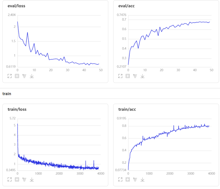
经过50个epochs的训练,训练集和验证集的Accuracy和Loss的实时变化趋势如下。虽然模型还未收敛,但是验证集的准确率始终比训练集低,发生了过拟合(Overfitting)现象,最终的结果如下:
- 训练集:loss: 1.5264 - acc: 0.7980
- 验证集:loss: 0.7211 - acc: 0.6793
4.3 模型存储
将我们训练得到的模型进行保存,以便后续评估和测试使用。
model_1.save("model_1_food11/final")
5 模型评估和测试
5.1 预测测试
5.1.1 测试数据集
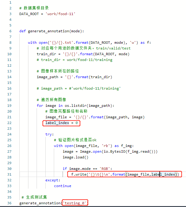
这里需要说明的是由于测试集没有标签,就不能直接进行实例化,即不能使用ZodiacDataset函数。在标注的时候将其图片路径全部补为0,才能进行预测。因为这对结果是没有影响的,实例化只是对测试集的图片进行处理。具体修改见下图:
from dataset import ZodiacDataset
testing_dataset = ZodiacDataset(mode='testing_0')
print('测试数据集样本量:{}'.format(len(testing_dataset)))
测试数据集样本量:3347
5.1.2 执行预测
from paddle.static import InputSpec
# 网络结构示例化
network =  ResNet18_1()
# 模型封装
model_2 = paddle.Model(network, inputs=[InputSpec(shape=[-1] + get('image_shape'), dtype='float64', name='image')])
# 训练好的模型加载
model_2.load('model_1_food11/final')
# 模型配置
model_2.prepare()
# 执行预测
result = model_2.predict(testing_dataset)
Predict begin...
step    2/3347 [..............................] - ETA: 8:12 - 147ms/step
/opt/conda/envs/python35-paddle120-env/lib/python3.7/site-packages/paddle/fluid/layers/utils.py:77: DeprecationWarning: Using or importing the ABCs from 'collections' instead of from 'collections.abc' is deprecated, and in 3.8 it will stop working
  return (isinstance(seq, collections.Sequence) and
step 3347/3347 [==============================] - 129ms/step
Predict samples: 3347
from PIL import Image
def openimg():  # 读取图片函数
    with open(f'work/food-11/testing.txt') as f:  #读取文件夹,这里读取的是没有标签的测试集
        txt =  []
        for line in f.readlines():  # 循环读取每一行
            txt.append(line[:-1])  # 生成列表
        return txt               #图片存放地址列表
# 读取图片存放路径列表
img_path = openimg()
# img_path[1],img_path[2000],img_path[3333],img_path[0],# 这条语句执行了下面的会出错,下次就不要执行。
('work/food-11/testing/0846.jpg',
 'work/food-11/testing/0457.jpg',
 'work/food-11/testing/2939.jpg',
 'work/food-11/testing/2235.jpg')
import matplotlib.pyplot as plt
from config import get
%matplotlib inline
# 随机取样本展示,测试数据集样本量:3347
# 样本映射
LABEL_MAP = get('LABEL_MAP')
indexs = [2,300,500, 666,862,999, 1102,1498,1532,1600,1775,1820,1912,2004,2459,2500,2601,2799,2905,3033,3334]

for idx in indexs:
    predict_label = np.argmax(result[0][idx])
    print('样本ID:{}, 预测标签:{}: {}'.format(idx,predict_label,LABEL_MAP[predict_label]))
    image = Image.open(img_path[idx])
    plt.figure(figsize=(10,6))
    plt.imshow(image)
    plt.title('predict: {}'.format(predict_label))
    plt.show()
随机抽取21张测试集预测的结果可视化出来,可以根据预测的中文标签对比图片就知道对错了。
样本ID:2, 预测标签:9: 汤

样本ID:300, 预测标签:3: 鸡蛋

样本ID:500, 预测标签:3: 鸡蛋

样本ID:666, 预测标签:0: 面包

样本ID:862, 预测标签:2: 甜点

样本ID:999, 预测标签:3: 鸡蛋

样本ID:1102, 预测标签:2: 甜点

样本ID:1498, 预测标签:7: 米饭

样本ID:1532, 预测标签:5: 肉类

样本ID:1600, 预测标签:10: 蔬菜or水果

样本ID:1775, 预测标签:10: 蔬菜or水果

样本ID:1820, 预测标签:9: 汤

样本ID:1912, 预测标签:9: 汤

样本ID:2004, 预测标签:0: 面包

样本ID:2459, 预测标签:6: 面条or意大利面

样本ID:2500, 预测标签:4: 油炸食品

样本ID:2601, 预测标签:0: 面包

样本ID:2799, 预测标签:6: 面条or意大利面

样本ID:2905, 预测标签:0: 面包

样本ID:3033, 预测标签:2: 甜点

样本ID:3334, 预测标签:8: 海鲜(最后一张未显示出来)
5.2 模型评价
由于测试集的标签没有给出,但可以通过批量预测并可视化展示就能大概知道模型是否好坏了。从上面展示的批量预测结果看,模型的预测准确率还是可以的,还需要继续学习会得到更高的准确率。
6 模型部署
# 保存模型用于部署
model_2.save('infer/food11', training=False)
7 残差神经网络搭建的方法
通过调整模块内部Residual的数量和配置实现不同的 ResNet,如resnet18是[2,2,2,2],如resnet34是[3,4,6,3]。通过改变下述三个参数可以得到不同的残差神经网络。
方法如下图:
8 参考文献&文章&代码
(1)飞桨官方教程&API
(2)https://blog.youkuaiyun.com/weixin_45623093/article/details/114490181
(3)龙龙老师教材:TensorFlow深度学习,P267-p274. 官方视频传送门
(4)https://blog.youkuaiyun.com/weixin_44331304/article/details/106127552
(5)https://aistudio.baidu.com/aistudio/projectdetail/1511752
(6)https://aistudio.baidu.com/aistudio/projectdetail/1354419
作者介绍
大家好,我是黄波波。希望能和大家共进步,错误之处恳请指出!
百度AI Studio个人主页, 我在AI Studio上获得白银等级,点亮2个徽章,来互关呀~
交流qq:3207820044
附录
以下两个文件为附加的文件,将其创建为py文件然后放在同一目录下即可。
# config.py文件,内部参数可变
__all__ = ['CONFIG', 'get']

CONFIG = {
    'model_save_dir': "./output/zodiac",
    'num_classes': 11,
    'total_images': 9866,
    'epochs': 50,
    'batch_size': 128,
    'image_shape': [3, 224, 224],
    'LEARNING_RATE': {
        'params': {
            'lr': 0.00375
        }
    },
    'OPTIMIZER': {
        'params': {
            'momentum': 0.90
        },
        'regularizer': {
            'function': 'L2',
            'factor': 0.000001
        }
    },
    'LABEL_MAP': [
        "面包",
        "乳制品",
        "甜点",
        "鸡蛋",
        "油炸食品",
        "肉类",
        "面条or意大利面",
        "米饭",
        "海鲜",
        "汤",
        "蔬菜or水果",
    ]
}
def get(full_path):
    for id, name in enumerate(full_path.split('.')):
        if id == 0:
            config = CONFIG

        config = config[name]

    return config
# data.py文件,内部参数可变
import paddle
import paddle.vision.transforms as T
import numpy as np
from config import get
from PIL import Image

__all__ = ['ZodiacDataset']

# 定义图像的大小
image_shape = get('image_shape')
IMAGE_SIZE = (image_shape[1], image_shape[2]) # [224,224]
class ZodiacDataset(paddle.io.Dataset):
    """
    数据集类的定义
    """

    def __init__(self, mode='training'):
        """
        初始化函数
        """
        assert mode in ['training', 'validation'], 'mode is one of train,  valid.'

        self.data = []

        with open('work/food-11/{}.txt'.format(mode)) as f:
            for line in f.readlines():
                info = line.strip().split('\t')

                if len(info) > 1:
                    self.data.append([info[0].strip(), info[1].strip()])

        if mode == 'training':
            self.transforms = T.Compose([
                T.Resize((256,256)),
                T.RandomCrop(IMAGE_SIZE),
                T.RandomRotation(15),    # 随机裁剪大小[224,224]
                T.RandomHorizontalFlip(0.5), # 随机水平翻转
                T.RandomVerticalFlip(0.5),       # 随机垂直翻转
                T.ToTensor(),                       # 数据的格式转换和标准化 HWC => CHW
                T.Normalize(mean=[0.485, 0.456, 0.406], std=[0.229, 0.224, 0.225])  # 图像归一化
            ])
        else:
            self.transforms = T.Compose([
                T.Resize((256,256)),                 # 图像大小修改
                T.RandomCrop(IMAGE_SIZE),      # 随机裁剪
                T.ToTensor(),                  # 数据的格式转换和标准化 HWC => CHW
                T.Normalize(mean=[0.485, 0.456, 0.406], std=[0.229, 0.224, 0.225])   # 图像归一化
            ])

    def __getitem__(self, index):
        """
        根据索引获取单个样本
        """
        image_file, label = self.data[index]
        image = Image.open(image_file)

        if image.mode != 'RGB':
            image = image.convert('RGB')

        image = self.transforms(image)

        return image, np.array(label, dtype='int64')

    def __len__(self):
        """
        获取样本总数
        """
个样本
        """
        image_file, label = self.data[index]
        image = Image.open(image_file)

        if image.mode != 'RGB':
            image = image.convert('RGB')

        image = self.transforms(image)

        return image, np.array(label, dtype='int64')

    def __len__(self):
        """
        获取样本总数
        """
        return len(self.data)


 被折叠的 条评论
为什么被折叠?
被折叠的 条评论
为什么被折叠?
 到【灌水乐园】发言


