


1. 简介
1.1 定义
- 2008年WesMcKinney开发出的库
- 专门用于数据挖掘的开源python库
- 以Numpy为基础,借力Numpy模块在计算方面性能高的优势
- 基于matplotlib,能够简便的画图
- 独特的数据结构
1.2 优势
- Numpy能够处理数据,并且结合matplotlib解决部分数据展示等问题,但Pandas
- 增强图表可读性
-
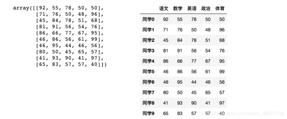
numpy创建学生成绩表样式:
-
返回结果:
import numpy as np
score = np.array([[92, 55, 78, 50, 50],
       [71, 76, 50, 48, 96],
       [45, 84, 78, 51, 68],
       [81, 91, 56, 54, 76],
       [86, 66, 77, 67, 95],
       [46, 86, 56, 61, 99],
       [46, 95, 44, 46, 56],
       [80, 50, 45, 65, 57],
       [41, 93, 90, 41, 97],
       [65, 83, 57, 57, 40]])
score
- 数据展示为这样,可读性就会更友好:
- 便捷的数据处理能力
- 读取文件方便
- 封装了Matplotlib、Numpy的画图和计算
1.3 作用
- 可以实现数据加载,清洗,转换,统计处理,可视化等功能
2. Pandas数据结构
Pandas中一共有三种数据结构,分别为:Series、DataFrame和MultiIndex(老版本中叫Panel )。
其中Series是一维数据结构,DataFrame是二维的表格型数据结构,MultiIndex是三维的数据结构。
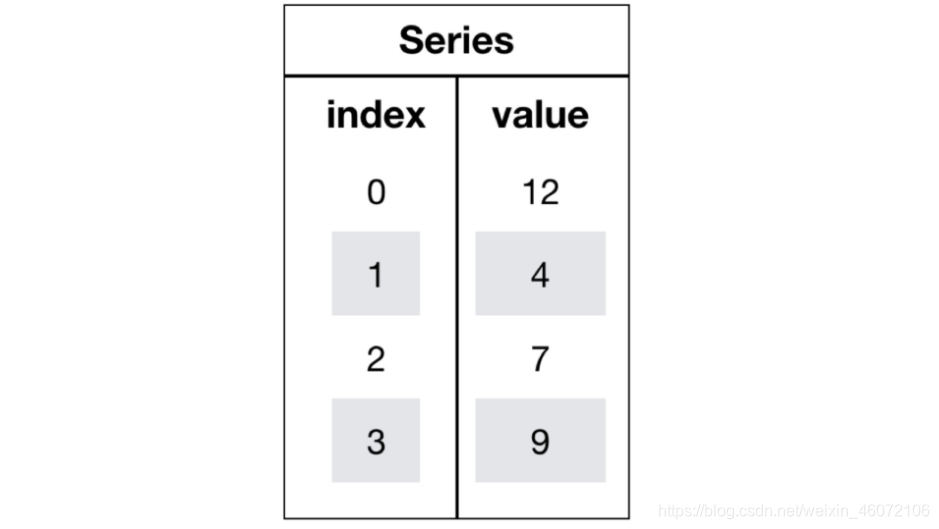
2.1 Series
1. 简介
- Series是一个类似于一维数组的数据结构,它能够保存任何类型的数据,比如整数、字符串、浮点数等,主要由一组数据和与之相关的索引两部分构成。
2. 操作
2.1 创建
# 导入pandas
import pandas as pd

pd.Series(data=None, index=None, dtype=None)
- 参数:
- data:传入的数据,可以是ndarray、list等
- index:索引,必须是唯一的,且与数据的长度相等。如果没有传入索引参数,则默认会自动创建一个从0-N的整数索引。
- dtype:数据的类型
通过已有数据创建
- 指定内容,默认索引
pd.Series(np.arange(10))
- 指定索引
pd.Series([6.7,5.6,3,10,2], index=[1,2,3,4,5])
- 通过字典数据创建
color_count = pd.Series({'red':100, 'blue':200, 'green': 500, 'yellow':1000})
color_count
2.2 属性
- 为了更方便地操作Series对象中的索引和数据,Series中提供了两个属性index和values
- index
color_count.index
- values
color_count.values
也可以使用索引来获取数据:
color_count[2]
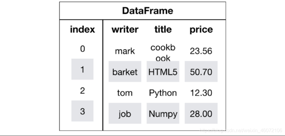
2.2 DataFrame
1. 定义
- DataFrame是一个类似于二维数组或表格(如excel)的对象,既有行索引,又有列索引
- 行索引,表明不同行,横向索引,叫index,0轴,axis=0
- 列索引,表名不同列,纵向索引,叫columns,1轴,axis=1
2. 创建
# 导入pandas
import pandas as pd

pd.DataFrame(data=None, index=None, columns=None)
- 参数:
- index:行标签。如果没有传入索引参数,则默认会自动创建一个从0-N的整数索引。
- columns:列标签。如果没有传入索引参数,则默认会自动创建一个从0-N的整数索引。
通过已有数据创建
举例一:
pd.DataFrame(np.random.randn(2,3))
- 使用np创建的数组显示方式,比较两者的区别。
举例二:创建学生成绩表
# 生成10名同学,5门功课的数据
score = np.random.randint(40, 100, (10, 5))
score
-
数据形式很难看到存储的是什么的样的数据,可读性比较差
-
让数据更有意义的显示
# 使用Pandas中的数据结构
score_df = pd.DataFrame(score)

- 给分数数据增加行列索引,显示效果更佳
效果:

- 增加行、列索引
# 构造行索引序列
subjects = ["语文", "数学", "英语", "政治", "体育"]

# 构造列索引序列
stu = ['同学' + str(i) for i in range(score_df.shape[0])]

# 添加行索引
data = pd.DataFrame(score, columns=subjects, index=stu)
data
3. 属性
- shape–形状
data.shape
- index–行索引
- DataFrame的行索引列表
data.index
- columns–列索引列表
data.columns
- values–查看值
- 直接获取其中array的值
data.values
- T–转置
data.T
- head(5):查看头部内容,显示前5行内容
如果不补充参数,默认5行。填入参数N则显示前N行
data.head(5)
- tail(5):查看尾部内容,显示后5行内容
如果不补充参数,默认5行。填入参数N则显示后N行
data.tail(5)
4. 索引的设置
需求:

1. 修改行列索引值
- 修改的时候,需要进行全局修改
stu = ["学生_" + str(i) for i in range(score_df.shape[0])]

# 必须整体全部修改
data.index = stu
注意:以下修改方式是错误的
# 错误修改方式
data.index[3] = '学生_3'
2. 重设索引
- reset_index(drop=False)
- 设置新的下标索引
- drop:默认为False,不删除原来索引,如果为True,删除原来的索引值
# 重置索引,drop=False
data.reset_index()
# 重置索引,drop=True
data.reset_index(drop=True)
3. 以某列值设置为新的索引
set_index(keys, drop=True)- keys : 列索引名成或者列索引名称的列表
- drop : boolean, default True.当做新的索引,删除原来的列
设置新索引案例
3.1 创建
df = pd.DataFrame({'month': [1, 4, 7, 10],
                    'year': [2012, 2014, 2013, 2014],
                    'sale':[55, 40, 84, 31]})
df
3.2 以月份设置新的索引
df.set_index('month')
3.3 设置多个索引,以年和月份
df = df.set_index(['year', 'month'])
df
注:通过刚才的设置,这样DataFrame就变成了一个具有MultiIndex的DataFrame。
2.3 MultiIndex与Panel
1. MultiIndex
1.1 简介
-
MultiIndex是三维的数据结构;
-
多级索引(也称层次化索引)是pandas的重要功能,可以在Series、DataFrame对象上拥有2个以及2个以上的索引。
-
类似ndarray中的三维数组
1.2 属性
对象.index
打印刚才的df的行索引结果
df.index
多级或分层索引对象。
- index属性
- names:levels的名称
- levels:每个level的元组值
df.index.names
df.index.levels
1.3 创建
- 语法:
pd.MultiIndex.from_arrays()
arrays = [[1, 1, 2, 2], ['red', 'blue', 'red', 'blue']]
pd.MultiIndex.from_arrays(arrays, names=('number', 'color'))
2. Panel
2.1 创建
pd.Panel(data, items, major_axis, minor_axis)
-
class
pandas.Panel(data=None, items=None, major_axis=None, minor_axis=None)-
作用:存储3维数组的Panel结构
-
参数:
-
data : ndarray或者dataframe
-
items : 索引或类似数组的对象,axis=0
-
major_axis : 索引或类似数组的对象,axis=1
-
minor_axis : 索引或类似数组的对象,axis=2
-
-
p = pd.Panel(data=np.arange(24).reshape(4,3,2),
                 items=list('ABCD'),
                 major_axis=pd.date_range('20130101', periods=3),
                 minor_axis=['first', 'second'])

# 结果
<class 'pandas.core.panel.Panel'>
Dimensions: 4 (items) x 3 (major_axis) x 2 (minor_axis)
Items axis: A to D
Major_axis axis: 2013-01-01 00:00:00 to 2013-01-03 00:00:00
Minor_axis axis: first to second
2.2 查看panel数据
- panel数据要是想看到,则需要进行索引到dataframe或者series才可以
p[:,:,"first"]
p["B",:,:]
注:Pandas从版本0.20.0开始弃用:推荐的用于表示3D数据的方法是通过DataFrame上的MultiIndex方法
3. 基本数据操作
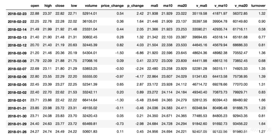
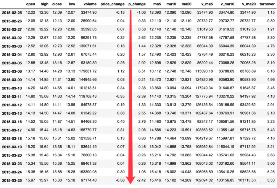
- 读取一个真实的股票数据。
# 读取文件
data = pd.read_csv("./data/stock_day.csv")

# 删除一些列,让数据更简单些,再去做后面的操作
data = data.drop(["ma5","ma10","ma20","v_ma5","v_ma10","v_ma20"], axis=1)
3.1 索引
- Numpy可以使用索引选取序列和切片选择,pandas也支持类似的操作,也可以直接使用列名、行名称,甚至组合使用。
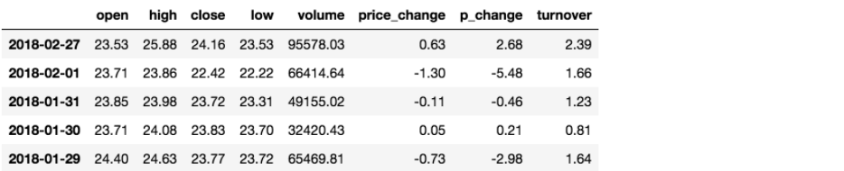
1. 直接使用行列索引(先列后行)
获取’2018-02-27’这天的’open’的结果
# 直接使用行列索引名字的方式(先列后行)
data['open']['2018-02-27']
23.53

# 不支持的操作
# 错误
data['2018-02-27']['open']
# 错误
data[:1, :2]
2. 结合loc或者iloc使用索引
- loc – 先行后列,是需要通过索引的字符串进行获取
- iloc – 先行后列,是通过下标进行索引
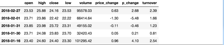
获取从’2018-02-27’:‘2018-02-22’,'open’的结果
# 使用loc:只能指定行列索引的名字
data.loc['2018-02-27':'2018-02-22', 'open']

2018-02-27    23.53
2018-02-26    22.80
2018-02-23    22.88
Name: open, dtype: float64

# 使用iloc可以通过索引的下标去获取
# 获取前3天数据,前5列的结果
data.iloc[:3, :5]

            open    high    close    low
2018-02-27    23.53    25.88    24.16    23.53
2018-02-26    22.80    23.78    23.53    22.80
2018-02-23    22.88    23.37    22.82    22.71
3. 使用ix组合索引
Warning:Starting in 0.20.0, the .ix indexer is deprecated, in favor of the more strict .iloc and .loc indexers.
- ix – 先行后列, 可以用上面两种方法混合进行索引
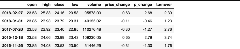
获取行第1天到第4天,[‘open’, ‘close’, ‘high’, ‘low’]这个四个指标的结果
# 使用ix进行下表和名称组合做引
data.ix[0:4, ['open', 'close', 'high', 'low']]

# 推荐使用loc和iloc来获取的方式
data.loc[data.index[0:4], ['open', 'close', 'high', 'low']]
data.iloc[0:4, data.columns.get_indexer(['open', 'close', 'high', 'low'])]

            open    close    high    low
2018-02-27    23.53    24.16    25.88    23.53
2018-02-26    22.80    23.53    23.78    22.80
2018-02-23    22.88    22.82    23.37    22.71
2018-02-22    22.25    22.28    22.76    22.02
3.2 赋值
data[""] = **
data. =
对DataFrame当中的close列进行重新赋值为1
# 直接修改原来的值
data['close'] = 1
# 或者
data.close = 1
3.3 排序
排序有两种形式,一种对于索引进行排序,一种对于内容进行排序
- dataframe
- 对象.sort_values()
- 对象.sort_index()
- series
- 对象.sort_values()
- 对象.sort_index()
1. DataFrame排序
- 使用df.sort_values(by=, ascending=)
- 单个键或者多个键进行排序,
- 参数:
- by:指定排序参考的键
- ascending:默认升序
- ascending=False:降序
- ascending=True:升序
# 按照开盘价大小进行排序 , 使用ascending指定按照大小排序
data.sort_values(by="open", ascending=True).head()
# 按照多个键进行排序
data.sort_values(by=['open', 'high'])
- 使用df.sort_index给索引进行排序
这个股票的日期索引原来是从大到小,现在重新排序,从小到大
# 对索引进行排序
data.sort_index()
2. Series排序
- 使用series.sort_values(ascending=True)进行排序
series排序时,只有一列,不需要参数
data['p_change'].sort_values(ascending=True).head()

2015-09-01   -10.03
2015-09-14   -10.02
2016-01-11   -10.02
2015-07-15   -10.02
2015-08-26   -10.01
Name: p_change, dtype: float64
- 使用series.sort_index()进行排序
与df一致
# 对索引进行排序
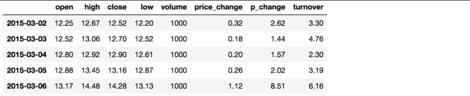
data['p_change'].sort_index().head()
2015-03-02 2.62
2015-03-03 1.44
2015-03-04 1.57
2015-03-05 2.02
2015-03-06 8.51
Name: p_change, dtype: float64
4. DataFrame运算
4.1 算术运算
- add(other)
- sub(other)’
比如进行数学运算加上具体的一个数字
data['open'].add(1)

2018-02-27    24.53
2018-02-26    23.80
2018-02-23    23.88
2018-02-22    23.25
2018-02-14    22.49
4.2 逻辑运算
1. 逻辑运算符号
- 例如筛选data[“open”] > 23的日期数据
- data[“open”] > 23返回逻辑结果
data["open"] > 23

2018-02-27     True
2018-02-26    False
2018-02-23    False
2018-02-22    False
2018-02-14    False
# 逻辑判断的结果可以作为筛选的依据
data[data["open"] > 23].head()
- 完成多个逻辑判断
data[(data["open"] > 23) & (data["open"] < 24)].head()
2. 逻辑运算函数
- query(expr)
- expr:查询字符串
data.query("open<24 & open>23").head()
- isin(values)
例如判断’open’是否为23.53和23.85
# 可以指定值进行一个判断,从而进行筛选操作
data[data["open"].isin([23.53, 23.85])]
4.3 统计运算
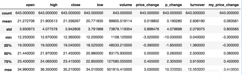
1. describe
综合分析: 能够直接得出很多统计结果,count, mean, std, min, max等
# 计算平均值、标准差、最大值、最小值
data.describe()
2. 统计函数
min(最小值), max(最大值), mean(平均值), median(中位数), var(方差), std(标准差),mode(众数)结果:
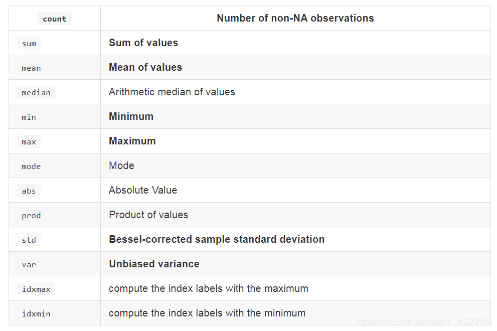
对于单个函数去进行统计的时候,坐标轴还是按照默认列“columns” (axis=0, default),如果要对行“index” 需要指定(axis=1)
- max()、min()
# 使用统计函数:0 代表列求结果, 1 代表行求统计结果
data.max(0)

open                   34.99
high                   36.35
close                  35.21
low                    34.01
volume             501915.41
price_change            3.03
p_change               10.03
turnover               12.56
my_price_change         3.41
dtype: float64
- std()、var()
# 方差
data.var(0)

open               1.545255e+01
high               1.662665e+01
close              1.554572e+01
low                1.437902e+01
volume             5.458124e+09
price_change       8.072595e-01
p_change           1.664394e+01
turnover           4.323800e+00
my_price_change    6.409037e-01
dtype: float64

# 标准差
data.std(0)

open                   3.930973
high                   4.077578
close                  3.942806
low                    3.791968
volume             73879.119354
price_change           0.898476
p_change               4.079698
turnover               2.079375
my_price_change        0.800565
dtype: float64
- median():中位数
中位数为将数据从小到大排列,在最中间的那个数为中位数。如果没有中间数,取中间两个数的平均值。
df = pd.DataFrame({'COL1' : [2,3,4,5,4,2],
                   'COL2' : [0,1,2,3,4,2]})

df.median()

COL1    3.5
COL2    2.0
dtype: float64
- idxmax()、idxmin()
# 求出最大值的位置
data.idxmax(axis=0)

open               2015-06-15
high               2015-06-10
close              2015-06-12
low                2015-06-12
volume             2017-10-26
price_change       2015-06-09
p_change           2015-08-28
turnover           2017-10-26
my_price_change    2015-07-10
dtype: object


# 求出最小值的位置
data.idxmin(axis=0)

open               2015-03-02
high               2015-03-02
close              2015-09-02
low                2015-03-02
volume             2016-07-06
price_change       2015-06-15
p_change           2015-09-01
turnover           2016-07-06
my_price_change    2015-06-15
dtype: object
3. 累计统计函数
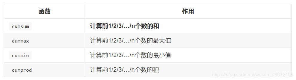
使用累计统计函数
以上这些函数可以对series和dataframe操作
按照时间的从前往后来进行累计
- 排序
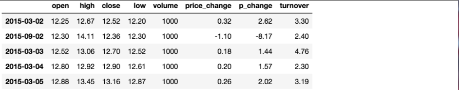
# 排序之后,进行累计求和
data = data.sort_index()
- 对p_change进行求和
stock_rise = data['p_change']
# plot方法集成了前面直方图、条形图、饼图、折线图
stock_rise.cumsum()

2015-03-02      2.62
2015-03-03      4.06
2015-03-04      5.63
2015-03-05      7.65
2015-03-06     16.16
2015-03-09     16.37
2015-03-10     18.75
2015-03-11     16.36
2015-03-12     15.03
2015-03-13     17.58
2015-03-16     20.34
2015-03-17     22.42
2015-03-18     23.28
2015-03-19     23.74
2015-03-20     23.48
2015-03-23     23.74
更好的显示连续求和的结果
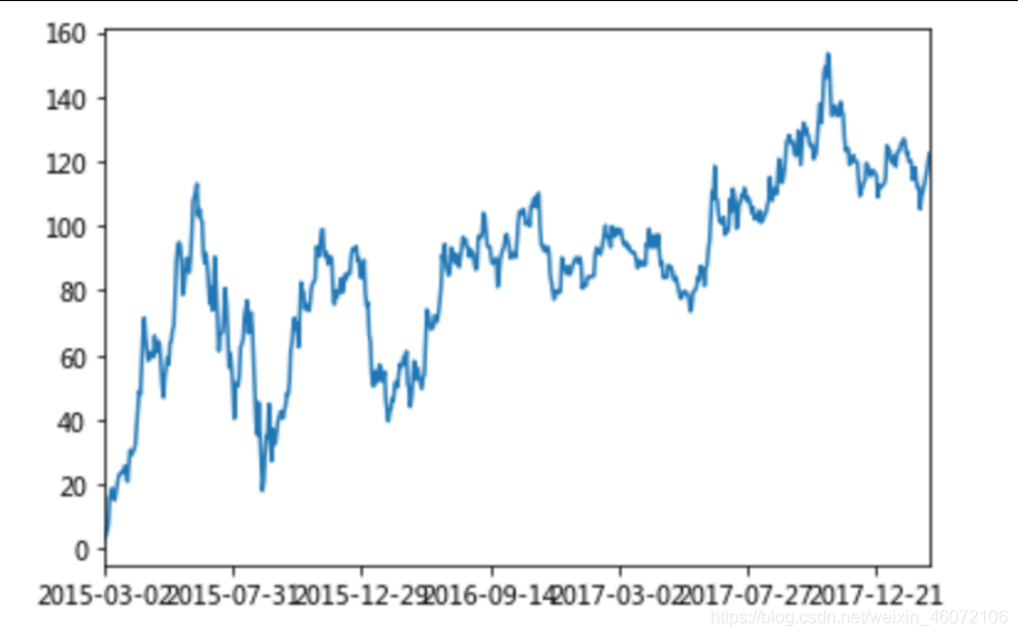
如果要使用plot函数,需要导入matplotlib.
import matplotlib.pyplot as plt
# plot显示图形
stock_rise.cumsum().plot()
# 需要调用show,才能显示出结果
plt.show()
4. 自定义运算
- apply(func, axis=0)
- func:自定义函数
- axis=0:默认是列,axis=1为行进行运算
- 定义一个对列,最大值-最小值的函数
data[['open', 'close']].apply(lambda x: x.max() - x.min(), axis=0)

open     22.74
close    22.85
dtype: float64
5. Pandas画图
5.1 pandas.DataFrame.plot
- DataFrame.plot(kind=‘line’)
- kind : str,需要绘制图形的种类
- ‘line’ : line plot (default)
- ‘bar’ : vertical bar plot
- ‘barh’ : horizontal bar plot
- ‘hist’ : histogram
- ‘pie’ : pie plot
- ‘scatter’ : scatter plot
5.2 pandas.Series.plot
6. 文件读取与存储
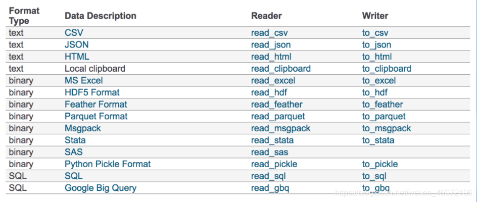
- 数据大部分存在于文件当中,所以pandas会支持复杂的IO操作,pandas的API支持众多的文件格式,如CSV、SQL、XLS、JSON、HDF5。
注:最常用的HDF5和CSV文件
6.1 CSV
1. read_csv
pandas.read_csv(filepath_or_buffer, sep =',', usecols )

filepath_or_buffer:文件路径
sep :分隔符,默认用","隔开
usecols:指定读取的列名,列表形式
举例:读取之前的股票的数据
# 读取文件,并且指定只获取'open', 'close'指标
data = pd.read_csv("./data/stock_day.csv", usecols=['open', 'close'])

            open    close
2018-02-27    23.53    24.16
2018-02-26    22.80    23.53
2018-02-23    22.88    22.82
2018-02-22    22.25    22.28
2018-02-14    21.49    21.92
2. to_csv
DataFrame.to_csv(path_or_buf=None, sep=', ’, columns=None, header=True, index=True, mode='w', encoding=None)

path_or_buf :文件路径
sep :分隔符,默认用","隔开
columns :选择需要的列索引
header :boolean or list of string, default True,是否写进列索引值
index:是否写进行索引
mode:'w':重写, 'a' 追加
举例:保存读取出来的股票数据
- 保存’open’列的数据,然后读取查看结果
# 选取10行数据保存,便于观察数据
data[:10].to_csv("./data/test.csv", columns=['open'])
# 读取,查看结果
pd.read_csv("./data/test.csv")

     Unnamed: 0    open
0    2018-02-27    23.53
1    2018-02-26    22.80
2    2018-02-23    22.88
3    2018-02-22    22.25
4    2018-02-14    21.49
5    2018-02-13    21.40
6    2018-02-12    20.70
7    2018-02-09    21.20
8    2018-02-08    21.79
9    2018-02-07    22.69
会发现将索引存入到文件当中,变成单独的一列数据。如果需要删除,可以指定index参数,删除原来的文件,重新保存一次。
# index:存储不会讲索引值变成一列数据
data[:10].to_csv("./data/test.csv", columns=['open'], index=False)
6.2 HDF5
1. read_hdf与to_hdf
HDF5文件的读取和存储需要指定一个键,值为要存储的DataFrame
pandas.read_hdf(path_or_buf,key =None,** kwargs)

从h5文件当中读取数据

path_or_buffer:文件路径
key:读取的键
return:Theselected object
DataFrame.to_hdf(path_or_buf, key, *\kwargs*)
2. 应用
- 读取文件
day_close = pd.read_hdf("./data/day_close.h5")
如果读取的时候出现以下错误
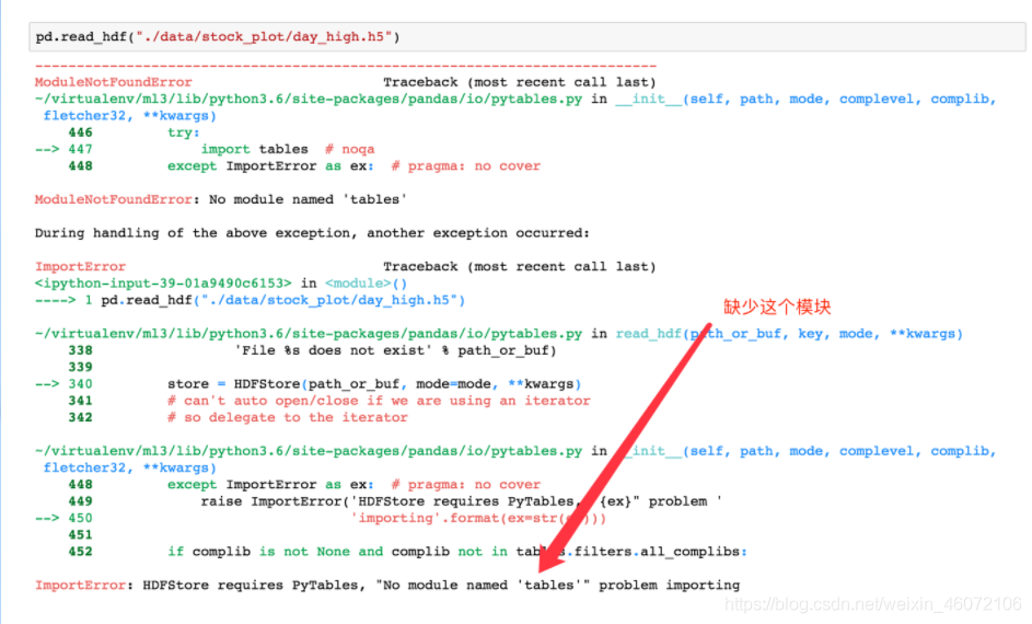
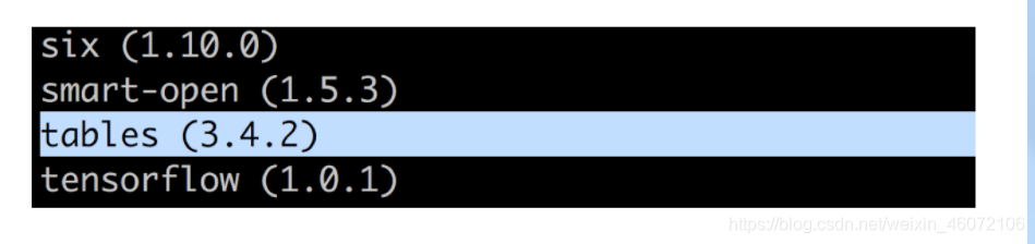
需要安装安装tables模块避免不能读取HDF5文件
pip install tables
- 存储文件
day_close.to_hdf("./data/test.h5", key="day_close")
再次读取的时候, 需要指定键的名字
new_close = pd.read_hdf("./data/test.h5", key="day_close")
注意:优先选择使用HDF5文件存储
- HDF5在存储的时候支持压缩,使用的方式是blosc,这个是速度最快的也是pandas默认支持的
- 使用压缩可以提磁盘利用率,节省空间
- HDF5还是跨平台的,可以轻松迁移到hadoop 上面
6.3 JSON
JSON是常用的一种数据交换格式,在前后端的交互经常用到,也会在存储的时候选择这种格式。
1. read_json
pandas.read_json(path_or_buf=None, orient=None, typ='frame', lines=False)

将JSON格式准换成默认的Pandas DataFrame格式
orient : string,Indication of expected JSON string format.
'split' : dict like {index -> [index], columns -> [columns], data -> [values]}
split 将索引总结到索引,列名到列名,数据到数据。将三部分都分开了
'records' : list like [{column -> value}, ... , {column -> value}]
records 以columns:values的形式输出
'index' : dict like {index -> {column -> value}}
index 以index:{columns:values}...的形式输出
'columns' : dict like {column -> {index -> value}},默认该格式
colums 以columns:{index:values}的形式输出
'values' : just the values array
values 直接输出值
lines : boolean, default False
按照每行读取json对象
typ : default ‘frame’, 指定转换成的对象类型series或者dataframe
2. 应用
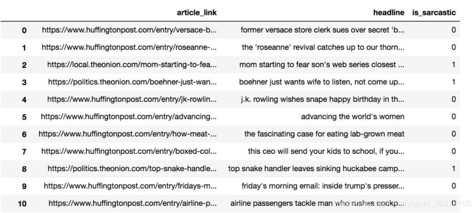
- 数据介绍
使用一个新闻标题讽刺数据集,格式为json。is_sarcastic:1讽刺的,否则为0;headline:新闻报道的标题;article_link:链接到原始新闻文章。存储格式为:
{"article_link": "https://www.huffingtonpost.com/entry/versace-black-code_us_5861fbefe4b0de3a08f600d5", "headline": "former versace store clerk sues over secret 'black code' for minority shoppers", "is_sarcastic": 0}
{"article_link": "https://www.huffingtonpost.com/entry/roseanne-revival-review_us_5ab3a497e4b054d118e04365", "headline": "the 'roseanne' revival catches up to our thorny political mood, for better and worse", "is_sarcastic": 0}
- 读取
orient指定存储的json格式,lines指定按照行去变成一个样本
json_read = pd.read_json("./data/Sarcasm_Headlines_Dataset.json", orient="records", lines=True)
结果为:
3. to_json
DataFrame.to_json(path_or_buf=None, orient=None, lines=False)
将Pandas 对象存储为json格式
path_or_buf=None:文件地址
orient:存储的json形式,{‘split’,’records’,’index’,’columns’,’values’}
lines:一个对象存储为一行
4. 应用
- 存储文件
json_read.to_json("./data/test.json", orient='records')
结果
[{"article_link":"https:\/\/www.huffingtonpost.com\/entry\/versace-black-code_us_5861fbefe4b0de3a08f600d5","headline":"former versace store clerk sues over secret 'black code' for minority shoppers","is_sarcastic":0},{"article_link":"https:\/\/www.huffingtonpost.com\/entry\/roseanne-revival-review_us_5ab3a497e4b054d118e04365","headline":"the 'roseanne' revival catches up to our thorny political mood, for better and worse","is_sarcastic":0},{"article_link":"https:\/\/local.theonion.com\/mom-starting-to-fear-son-s-web-series-closest-thing-she-1819576697","headline":"mom starting to fear son's web series closest thing she will have to grandchild","is_sarcastic":1},{"article_link":"https:\/\/politics.theonion.com\/boehner-just-wants-wife-to-listen-not-come-up-with-alt-1819574302","headline":"boehner just wants wife to listen, not come up with alternative debt-reduction ideas","is_sarcastic":1},{"article_link":"https:\/\/www.huffingtonpost.com\/entry\/jk-rowling-wishes-snape-happy-birthday_us_569117c4e4b0cad15e64fdcb","headline":"j.k. rowling wishes snape happy birthday in the most magical way","is_sarcastic":0},{"article_link":"https:\/\/www.huffingtonpost.com\/entry\/advancing-the-worlds-women_b_6810038.html","headline":"advancing the world's women","is_sarcastic":0},....]
- 修改lines参数为True
json_read.to_json("./data/test.json", orient='records', lines=True)
结果
{"article_link":"https:\/\/www.huffingtonpost.com\/entry\/versace-black-code_us_5861fbefe4b0de3a08f600d5","headline":"former versace store clerk sues over secret 'black code' for minority shoppers","is_sarcastic":0}
{"article_link":"https:\/\/www.huffingtonpost.com\/entry\/roseanne-revival-review_us_5ab3a497e4b054d118e04365","headline":"the 'roseanne' revival catches up to our thorny political mood, for better and worse","is_sarcastic":0}
{"article_link":"https:\/\/local.theonion.com\/mom-starting-to-fear-son-s-web-series-closest-thing-she-1819576697","headline":"mom starting to fear son's web series closest thing she will have to grandchild","is_sarcastic":1}
{"article_link":"https:\/\/politics.theonion.com\/boehner-just-wants-wife-to-listen-not-come-up-with-alt-1819574302","headline":"boehner just wants wife to listen, not come up with alternative debt-reduction ideas","is_sarcastic":1}
{"article_link":"https:\/\/www.huffingtonpost.com\/entry\/jk-rowling-wishes-snape-happy-birthday_us_569117c4e4b0cad15e64fdcb","headline":"j.k. rowling wishes snape happy birthday in the most magical way","is_sarcastic":0}...
### 2 加载数据集
import pandas as pd
df = pd.read_csv('xxxxx', sep='zzz')
shape是属性 显示形状
columns属性 显示列名
dtypes属性 查看列类型
df.info() 显示df的详细信息
Pandas与Python常用数据类型对照
pandas object就是python的str
### 3 查看部分数据
查看列数据
加载一列数据,通过df['列名']方式获取或者 df.列名
通过列名加载多列数据,通过df[['列名1','列名2',...]],**注意**多个列的列明放在list中传入
按行加载部分数据
loc[行索引] 获取行数据
head() tail()获取开始的行 结尾的行
loc:通过索引标签获取指定多行数据 df.loc[[0, 99, 999]]
iloc : 通过行号获取行数据
**需要注意的是,iloc传入的是索引的序号,loc是索引的标签**
获取指定行/列数据
- df.loc[[行],[列]] loc 只能接受行/列 的名字, 不能传入索引
- df.iloc[[行],[列]] iloc只能接受行/列的索引,不能传入行名,或者列名
在 iloc中使用切片语法获取几列数据
subset = df.iloc[:,3:6]
使用 loc/iloc 获取指定行,指定列的数据
df.loc[42,'country']

### 4 分组和聚合计算
df.groupby('year')['lifeExp'].mean()
df.groupby(['year', 'continent'])[['lifeExp','gdpPercap']].mean()
reset_index方法(重置行索引)
multi_group_var = df.groupby(['year', 'continent'])[['lifeExp','gdpPercap']].mean()
flat = multi_group_var.reset_index()
分组统计数量
df.groupby('continent')['country'].nunique()
画图
global_yearly_life_expectancy.plot()
## 3 Pandas 数据结构
### 1 创建Series
s = pd.Series(['banana',42])
s = pd.Series(['Wes McKinney','Male'],index = ['Name','Gender'])
### 2 创建Dataframe
pd.DataFrame(
{'Name':['Tome','Bob'],
'Occupation':['Teacher','IT Engineer'],
'age':[28,36]})
### 3 Series常用属性方法
可以通过 index 和 values属性获取行索引和值
data.keys()
Series常用方法
value_counts() 分组 统计 排序
通过count()方法可以返回有多少非空值
通过describe()方法打印描述信息
Series的布尔索引
ages[ages>ages.mean()]
手动创建布尔值列表
bool_values = [False,True,True,False,False,False,False,False]
ages[bool_values]
Series 的运算
Series和数值型变量计算时,变量会与Series中的每个元素逐一进行计算
ages+100
两个Series之间计算,如果Series元素个数相同,则将两个Series对应元素进行计算
元素个数不同的Series之间进行计算,会根据索引进行。索引不同的元素最终计算的结果会填充成缺失值,用NaN表示
Series之间进行计算时,数据会尽可能依据索引标签进行相互计算
## 4 DataFrame常用操作
size 元素个数
该数据集的维度
movie.ndim
shape 形状
len(movie)
count()统计每列非空值
movie.describe()
DataFrame的布尔索引,DataFrame也可以使用布尔索引获取数据子集。
movie[movie['duration']>movie['duration'].mean()]
DataFrame的运算
当DataFrame和数值进行运算时,DataFrame中的每一个元素会分别和数值进行运算
两个DataFrame之间进行计算,会根据索引进行对应计算
两个DataFrame数据条目数不同时,会根据索引进行计算,索引不匹配的会返回NaN
## 5 修改Dataframe
指定行索引
通过set_index指定
movie2 = movie.set_index('movie_title')
加载数据时指定
pd.read_csv('data/movie.csv', index_col='movie_title')
通过reset_index()方法可以重置索引
修改列名和行索引
movie.rename(index=idx_rename, columns=col_rename)
直接给index 和columns赋值
添加、删除、插入列
通过dataframe[列名]添加新列 添加在最后一列
调用drop方法删除列 axis=columns
使用insert()方法插入列 loc 新插入的列在所有列中的位置(0,1,2,3...) column=列名 value=值
## 6 导出和导入数据
1 pickle文件,二进制文件,读取速度快,不容易看懂
names.to_pickle('output/scientists_name.pickle')
pd.read_pickle('output/scientists_name.pickle')
2 csv文件
names.to_csv('output/scientists_name.csv')
scientists.to_csv('output/scientists_df.tsv',sep='\t') 可以自定义分隔符
3 Excel文件
pandas读写excel需要额外安装如下三个包
pip install -i https://pypi.tuna.tsinghua.edu.cn/simple xlwt
pip install -i https://pypi.tuna.tsinghua.edu.cn/simple openpyxl
pip install -i https://pypi.tuna.tsinghua.edu.cn/simple xlrd
scientists.to_excel('output/scientists_df.xlsx',sheet_name='scientists',index=False)

index一般设置为False


 625
625

 被折叠的 条评论
为什么被折叠?
被折叠的 条评论
为什么被折叠?
 到【灌水乐园】发言


