


七、电影数据分析
7.1 背景介绍
7.1.1实验背景
电影娱乐产业越发发达,投资商希望能从电影的各种数据中找到最可能赚钱的电影有什么特点。
数据介绍
- budget 预算
- genres 电影名数据
- homepage 网站主页
- id
- keywords 关键字
- original_language 语言
- original_title 标题
- overview 概述
- popularity 人气
- popularity 电影商
- production_countries 电影商拍摄地
- release_date 发布日期
- revenue 收入
- runtime 电影时长
- spoken_languages 电影语言
- status 状态
- status 标语
- title 标题
- vote_average 评分
- 评分人数
- movie_id 电影id
- title 标题
- cast 投票人信息
- crew 所有信息
7.2 载入数据
7.2.1 导入支持库
import pandas as pd
import numpy as np
import matplotlib.pyplot as plt
import json
7.2.3 设置中文标签显示
plt.rcParams['font.sans-serif']=['SimHei'] #用来正常显示中文标签
plt.rcParams['axes.unicode_minus']=False #用来正常显示负号
7.2.4 载入数据集
movies=pd.read_csv(r'../data/tmdb_5000_movies.csv',sep=',')
credit=pd.read_csv(r'../data/tmdb_5000_credits.csv',sep=',')
7.3 数据清洗
7.3.1 检查两个id列和title列是否真的相同
(movies['id']==credit['movie_id']).describe()
[外链图片转存失败,源站可能有防盗链机制,建议将图片保存下来直接上传(img-m8rXBfbQ-1629090102555)(Matplotlib基础课程.assets/Matplotlib_10_1.png)]
(movies['title']==credit['title']).describe()
[外链图片转存失败,源站可能有防盗链机制,建议将图片保存下来直接上传(img-2qFw2TAL-1629090102557)(Matplotlib基础课程.assets/Matplotlib_10_2.png)]
7.3.2 删除多余列
del credit['movie_id']
del credit['title']
del movies['homepage']
del movies['spoken_languages']
del movies['original_language']
del movies['original_title']
del movies['overview']
del movies['tagline']
del movies['status']
7.3.3 合并两个数据集
full_df=pd.concat([credit,movies],axis=1)#横向连接
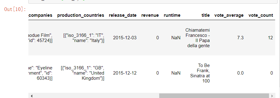
7.3.4 处理缺失值-首先找到缺失值
nan_x=full_df['runtime'].isnull()
full_df.loc[nan_x,:]
7.3.5 处理缺失值
full_df.loc[2656,'runtime']=98
full_df.loc[4140,'runtime']=82
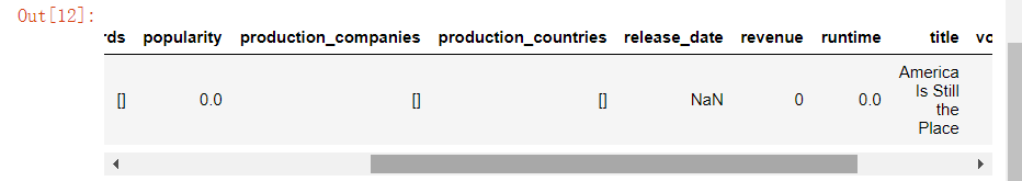
7.3.6 查找release_data的缺失值
nan_y=full_df['release_date'].isnull()
full_df.loc[nan_y,:]
7.3.7 处理release_data的缺失值
full_df.loc[4553,'release_date']='2014-06-01'
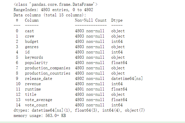
7.3.8 将release_date的类型转换成日期类型
full_df['release_date']=pd.to_datetime(full_df['release_date'],errors='coerce',format='%Y-%m-%d')
full_df.info()
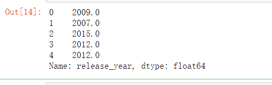
7.3.9 转换成日期格式后,提取对应的年份
full_df['release_year']=full_df['release_date'].map(lambda x : x.year)
full_df.loc[:,'release_year'].head()
7.3.10 处理json格式类型-提取json格式,使用json.loads将json格式转化成字符串
json_cols=['genres','keywords','production_companies','production_countries','cast','crew']
for i in json_cols:
full_df[i]=full_df[i].apply(json.loads)
def get_names(x):
return ','.join(i['name'] for i in x)
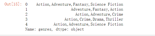
full_df['genres']=full_df['genres'].apply(get_names)
full_df['keywords']=full_df['keywords'].apply(get_names)
full_df['production_companies']=full_df['production_companies'].apply(get_names)
full_df['production_countries']=full_df['production_countries'].apply(get_names)
full_df['genres'].head()
7.3.11 获取所有电影类型
real_genres=set()
for i in full_df['genres'].str.split(','):
    real_genres=real_genres.union(i)
real_genres=list(real_genres)#将集合转换成列表
real_genres.remove('')#删除空格
print(real_genres)
[外链图片转存失败,源站可能有防盗链机制,建议将图片保存下来直接上传(img-bv5LlMku-1629090102565)(Matplotlib基础课程.assets/Matplotlib_10_8.png)]
7.3.12 将所有类型添加到列表
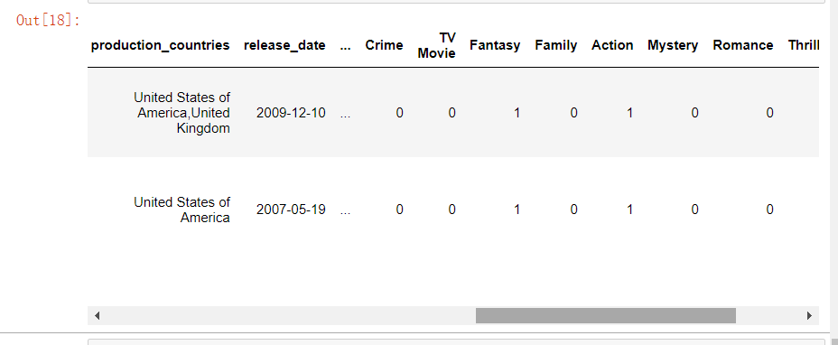
for i in real_genres:
  full_df[i]=full_df['genres'].str.contains(i).apply(lambda x:1 if x else 0)
full_df.head(2)
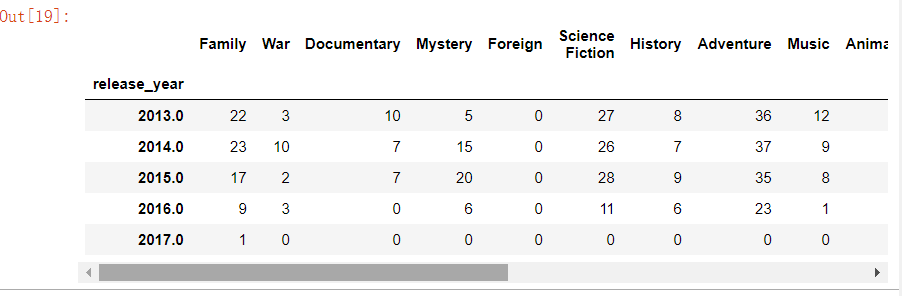
7.3.13 获取年份和类型子集,按年分组统计每年各类型电影数量
part1_df=full_df[['release_year', 'Family', 'War', 'Documentary', 'Mystery', 'Foreign','Science Fiction', 'History', 'Adventure', 'Music', 'Animation',
       'Western', 'Action', 'Crime', 'Comedy', 'Drama', 'Romance', 'Horror','Thriller', 'Fantasy', 'TV Movie']]

year_cnt=part1_df.groupby('release_year').sum()
year_cnt.tail()
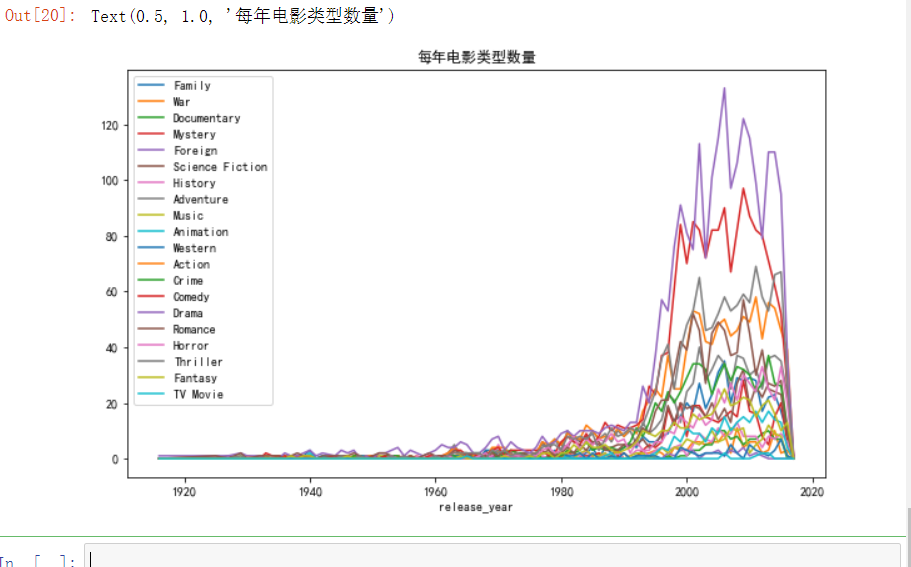
7.3.14 每年电影类别数量
plt.figure(figsize=(10,6))
plt.rc('font',family='SimHei',size=10)#设置字体和大小,否则中文无法显示
ax1=plt.subplot(1,1,1)
year_cnt.plot(kind='line',ax=ax1)
plt.title('每年电影类型数量')
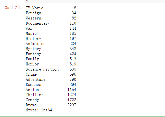
7.3.15 不同电影类型总数量
genre=year_cnt.sum(axis=0)#对列求和
genre=genre.sort_values(ascending=True)
genre
7.4 简单绘图分析
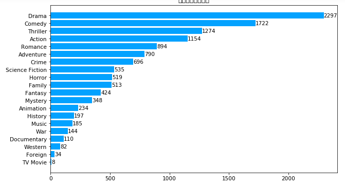
7.4.1 绘制分类数据横向条形图
plt.figure(figsize=(10,6))
plt.rc('font',family='STXihei',size=10.5)
ax2=plt.subplot(1,1,1)
label=list(genre.index)
data=genre.values
rect=ax2.barh(range(len(label)),data,color='#03A2FF',alpha=1)
ax2.set_title('不同电影类型数量')#设置标题
ax2.set_yticks(range(len(label)))
ax2.set_yticklabels(label)
#添加数据标签
for x,y in zip(data,range(len(label))):
    ax2.text(x,y,'{}'.format(x),ha='left',va='center')
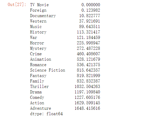
7.4.2 计算不同类型电影收入(亿元)
r={}
for i in real_genres:
    r[i]=full_df.loc[full_df[i]==1,'revenue'].sum(axis=0)/100000000
revenue=pd.Series(r).sort_values(ascending=True)
revenue
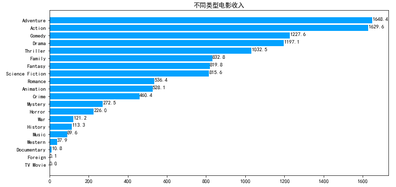
7.4.3 绘制电影收入的横向条形图
plt.figure(figsize=(12,6))
plt.rc('font',family='Simhei',size=10.5)
ax=plt.subplot(1,1,1)
label=revenue.index
data=revenue.values
ax.barh(range(len(label)),data,color='#03A2FF',alpha=1)
ax.set_yticks(range(len(label)))#设置y轴刻度
ax.set_yticklabels(label)#设置刻度名称
ax.set_title('不同类型电影收入')
#添加数据标签
for x,y in zip(data,range(len(label))):
    ax.text(x,y,'{:.1f}'.format(x))#坐标位置,及要显示的文字内容
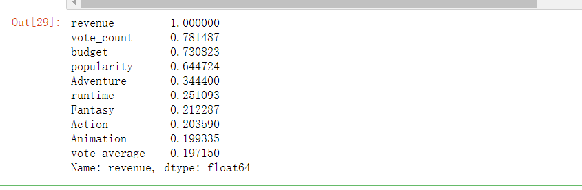
7.4.4 票房收入影响因素分析
corr=full_df.corr()#计算各变量间的相关系数矩阵
corr_revenue=corr['revenue'].sort_values(ascending=False)#提取收入与其他变量间的相关系数,并从大到小排序
corr_revenue.head(10)
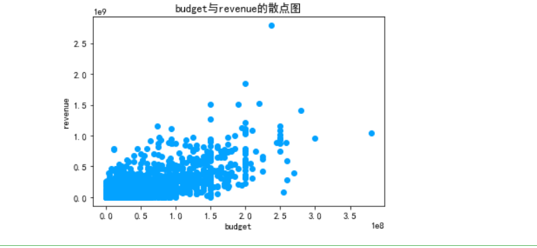
7.4.5 绘制散点图,分析budget与revenue的相关性
x=full_df.loc[:,'budget']
y=full_df.loc[:,'revenue']
plt.rc('font',family='SimHei',size=10.5)
plt.scatter(x,y,color='#03A2FF')
plt.xlabel('budget')
plt.ylabel('revenue')
plt.title('budget与revenue的散点图')
plt.show()
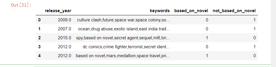
7.4.6 原创电影与改编电影分析
part2_df=full_df.loc[:,['release_year','keywords']]
part2_df['based_on_novel']=part2_df['keywords'].str.contains('based on novel').apply(lambda x:1 if x else 0)
part2_df['not_based_on_novel']=part2_df['keywords'].str.contains('based on novel').apply(lambda x:0 if x else 1)
part2_df.head()
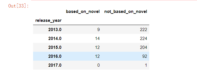
novel_per_year=part2_df.groupby('release_year')['based_on_novel','not_based_on_novel'].sum()
novel_per_year.tail()
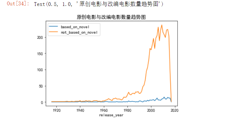
7.4.7 绘制原创电影与改变电影趋势图
novel_per_year.plot()
plt.rc('font',family='SimHei',size=10.5)
plt.title('原创电影与改编电影数量趋势图')
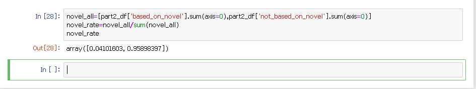
7.4.8 原创电影与改编电影总数
novel_all=[part2_df['based_on_novel'].sum(axis=0),part2_df['not_based_on_novel'].sum(axis=0)]
novel_rate=novel_all/sum(novel_all)
novel_rate
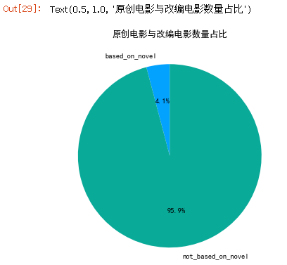
7.4.9 绘制原创电影和改编电影比例饼图
plt.figure(figsize=(6,6))
plt.rc('font',family='SimHei',size=10.5)
ax=plt.subplot(111)#与plt.sumplot(1,1,1)效果一样
labels=['based_on_novel','not_based_on_novel']
colors=['#03A2FF','#0AAA99']
ax.pie(novel_rate,labels=labels,colors=colors,startangle=90,autopct='%1.1f%%')
ax.set_title('原创电影与改编电影数量占比')
7.5 复杂绘图分析
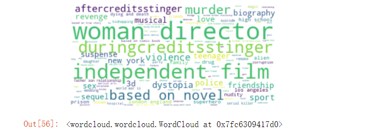
分析电影主题关进词
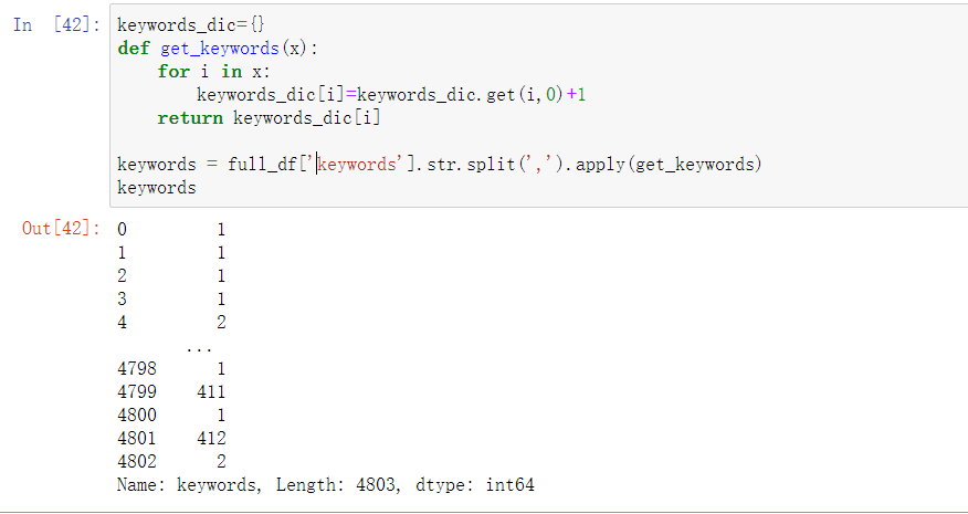
7.5.1 获取所有关键词及其对应词频
keywords_dic={}
def get_keywords(x):
    for i in x:
        keywords_dic[i]=keywords_dic.get(i,0)+1
    return keywords_dic[i]

keywords = full_df['keywords'].str.split(',').apply(get_keywords)
keywords
7.5.2 绘制词云图
安装wordcloud安装包:!pip install wordcloud
import matplotlib.pyplot as plt
from wordcloud import WordCloud,STOPWORDS
import pandas as pd

wordcloud=WordCloud(max_words=500 #最大词数
#                    ,font_path="DejaVuSerif.ttf"
#自定义字体
                    ,background_color="white" #背景颜色
                    ,max_font_size=80 #最大字号
                    ,prefer_horizontal=100 #词语水平方向排版出现的频率,设置为100表示全部水平显示
                    ,stopwords=STOPWORDS #使用屏蔽词
                    )
wordcloud=wordcloud.fit_words(keywords_dic)
plt.imshow(wordcloud)
plt.axis('off')
plt.show()
wordcloud.to_file('worldcloudt.jpg')
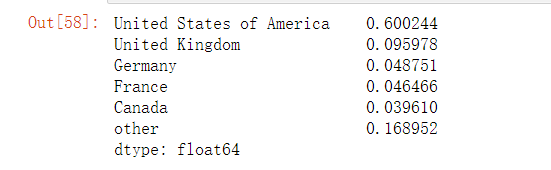
7.5.3 统计各个国家的电影数
part3_df=full_df[['production_countries','id','release_year']]#提取需要的列子集
#由于有的电影产地属于多个国家,故需要对production_countries进行分列
split_df=pd.DataFrame([x.split(',') for x in part3_df['production_countries']],index=part3_df.index)
#将分列后的数据集与源数据集合并
part3_df=pd.merge(part3_df,split_df,left_index=True,right_index=True)
#下面代码实现列转行
st_df=part3_df[['release_year',0,1,2,3]]
st_df=st_df.set_index('release_year')
st_df=st_df.stack()
st_df=st_df.reset_index()

st_df=st_df.rename(columns={0:'production_countries'})#对列重命名
countries=st_df['production_countries'].value_counts()#统计各个国家的电影数
countries.sum()
countries_rate=countries/countries.sum()#计算占比
countries_top5=countries_rate.head(5)
other={'other':1-countries_top5.sum()}
countries_top6=countries_top5.append(pd.Series(other))
countries_top6
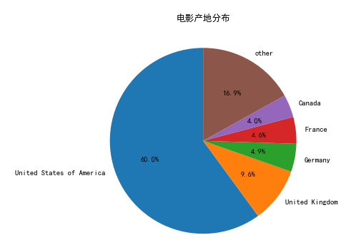
7.5.4 绘制安国家分类的电音出品饼图
labels=list(countries_top6.index)
plt.figure(figsize=(6,6))
plt.rc('font',family='SimHei',size=10.5)
ax=plt.subplot(1,1,1)
ax.pie(countries_top6,labels=labels,startangle=90,autopct='%1.1f%%')
ax.set_title('电影产地分布')
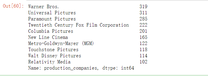
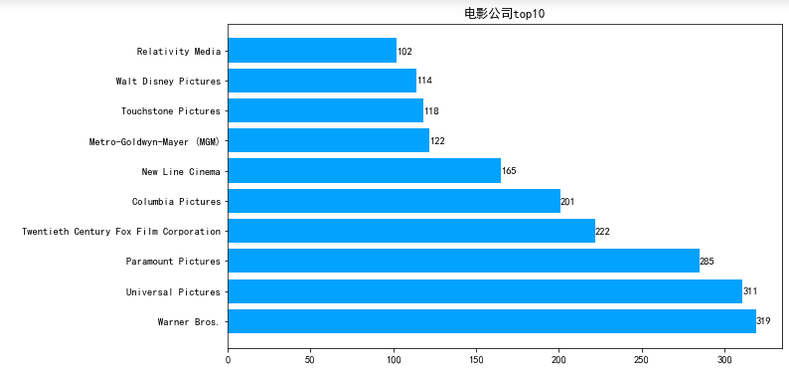
7.5.5 统计各个电影公司电影数
part4_df=full_df[['production_companies','release_year']]
split_df=pd.DataFrame([x.split(',') for x in part4_df['production_companies']],index=part4_df.index)
part4_df=pd.merge(part4_df,split_df,left_index=True,right_index=True)
del part4_df['production_companies']
part4_df=part4_df.set_index('release_year')
part4_df=part4_df.stack()
part4_df=part4_df.reset_index()
part4_df=part4_df.rename(columns={0:'production_companies'})
companies=part4_df['production_companies'].value_counts()
companies_top10=companies[companies.index!=''].head(10)
companies_top10
7.5.6 绘制电影公司条形图
plt.figure(figsize=(10,6))
plt.rc('font',family='SimHei',size=10.5)
ax=plt.subplot(111)
ax.barh(range(10),companies_top10.values,color='#03A2FF')
ax.set_title('电影公司top10')
ax.set_yticks(range(10))
ax.set_yticklabels(companies_top10.index)
for x,y in zip(companies_top10.values,range(10)):
    ax.text(x,y,'{}'.format(x),ha='left',va='center')


 6929
6929

 被折叠的 条评论
为什么被折叠?
被折叠的 条评论
为什么被折叠?
 到【灌水乐园】发言


