【GFPN代码解读】搭建图神经网络

首先我们可以从train文件中定位到我们搭建图神经网络的部分，位于graph_FeaturePyramid这个类中

1.graph_FeaturePyramid类（network.py）

我们忽略卷积层的搭建，直接来看图网络的搭建和传播

init初始化部分

self.context1 = contextual_layers(256, 256)   详见1.1
self.context2 = contextual_layers(256, 256)
self.context3 = contextual_layers(256, 256)
self.hierarch1 = hierarchical_layers(256, 256)  详见1.2
self.hierarch2 = hierarchical_layers(256, 256)
self.hierarch3 = hierarchical_layers(256, 256)
self.context4 = contextual_layers(256, 256)
self.context5 = contextual_layers(256, 256)
self.context6 = contextual_layers(256, 256)
self.g = simple_birected(build_edges(heterograph("pixel", 256, 1029))) 详见1.3，1.4
self.g = dgl.add_self_loop(self.g, etype = "hierarchical")
self.subg_h = hetero_subgraph(self.g, "hierarchical")   详见1.5
self.subg_c = hetero_subgraph(self.g, "contextual")

补充：
dgl.add_self_loop 是 DGL中的一个函数，用于为图添加自环边。
dgl.to_simple 是 DGL中的一个函数，用于将图转换为简单图，即移除重复边。
dgl.to_bidirected 函数将图转换为双向图，即为每条边添加反向边。

call部分

p_final = tf.concat([p3_gnn, p4_gnn, p5_gnn], axis = 0)
self.g = cnn_gnn(self.g, p_final)   详见2.1
nodes_update(self.subg_c, self.context1(self.subg_c, self.subg_c.ndata["pixel"]))
nodes_update(self.subg_c, self.context2(self.subg_c, self.subg_c.ndata["pixel"]))
nodes_update(self.subg_c, self.context3(self.subg_c, self.subg_c.ndata["pixel"]))
nodes_update(self.subg_h, self.hierarch1(self.subg_h, self.subg_h.ndata["pixel"]))
nodes_update(self.subg_h, self.hierarch2(self.subg_h, self.subg_h.ndata["pixel"]))
nodes_update(self.subg_h, self.hierarch3(self.subg_h, self.subg_h.ndata["pixel"]))
nodes_update(self.subg_c, self.context4(self.subg_c, self.subg_c.ndata["pixel"]))
nodes_update(self.subg_c, self.context5(self.subg_c, self.subg_c.ndata["pixel"]))
nodes_update(self.subg_c, self.context6(self.subg_c, self.subg_c.ndata["pixel"]))
# data fusion 
p3_gnn, p4_gnn, p5_gnn = gnn_cnn(self.g)  详见2.2

---

1.1 contextual_layers（network.py）

class contextual_layers(keras.layers.Layer):
def __init__(self, in_feats, h_feats, **kwarg):
     super().__init__(**kwarg)
     self.in_feats = in_feats
     self.gat1 = conv.GATConv(in_feats, h_feats, 1, activation=tf.nn.relu)
     self.gat2 = conv.GATConv(in_feats, h_feats, 1, activation=tf.nn.relu)
     self.gat3= conv.GATConv(in_feats, h_feats, 1, activation=tf.nn.relu)

 def call(self, g, in_feat):
     h = self.gat1(g, in_feat)
     h = self.gat2(g, h)
     h = self.gat3(g, h)
     h= tf.squeeze(h)
     return h

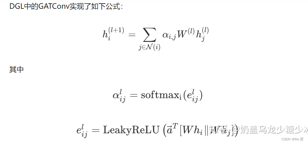
建了三个GATConv（Graph Attention Network）层，分别命名为gat1、gat2和gat3。
GATConv层通过计算节点之间的注意力系数，将每个节点的特征与其邻居节点的特征进行加权相加

GATConv接收8个参数：
- in_feats： int 或 int 对。如果是无向二部图，则in_feats表示(source node, destination node)的输入特征向量size；如果in_feats是标量，则source node=destination node。
- out_feats： int。输出特征size。
- num_heads： int。Multi-head Attention中heads的数量。
- feat_drop=0.： float。特征丢弃率。
- attn_drop=0.： float。注意力权重丢弃率。
- negative_slope=0.2： float。LeakyReLU的参数。
- residual=False： bool。是否采用残差连接。
- activation=None：用于更新后的节点的激活函数。

---

1.2 hierarchical_layers（network.py）

class hierarchical_layers(keras.layers.Layer):
def __init__(self, in_feats, h_feats, **kwarg):
   super().__init__(**kwarg)
   self.in_feats = in_feats
   self.gat1 = conv.GATConv(in_feats, h_feats, 1, activation=tf.nn.relu)
   self.gat2 = conv.GATConv(in_feats, h_feats, 1, activation=tf.nn.relu)
   self.gat3= conv.GATConv(in_feats, h_feats, 1, activation=tf.nn.relu)

def call(self, g, in_feat):
   h = self.gat1(g, in_feat)
   h = self.gat2(g, h)
   h = self.gat3(g, h)
   h = tf.squeeze(h)
   return h

与1.1的代码一致，故略过

---

1.3 heterograph（graph.py）

def heterograph(name_n_feature, dim_n_feature, nb_nodes = 2, is_birect = True):
    graph_data = {
        ('n', 'contextual', 'n'): (tf.constant([0]), tf.constant([1])),
        ('n', 'hierarchical', 'n'): (tf.constant([0]), tf.constant([1]))
        }
    g = dgl.heterograph(graph_data, num_nodes_dict = {'n': nb_nodes})
    g.nodes['n'].data[name_n_feature] = tf.zeros([g.num_nodes(), dim_n_feature])
    if is_birect:
        with tf.device("/cpu:0"):
            g = dgl.to_bidirected(g, copy_ndata = True)
        g = g.to("/gpu:0")
    return g

定义了一个名为graph_data的字典，它描述了异构图中的边关系
使用graph_data和节点数量参数nb_nodes创建了一个异构图g
将节点特征name_n_feature初始化为具有维度[g.num_nodes(), dim_n_feature]的全零张量
如果is_birect为True，将异构图转换为双向图，以增加边的反向连接
将异构图转移到GPU设备上，并将其作为函数的返回值

dgl.heterograph函数用于创建包含多个节点类型和边类型的异构图，接受一个字典参数graph_data，该字典描述了异构图中的边关系。

在上述代码中，graph_data字典定义了两种边类型：(‘n’, ‘contextual’, ‘n’)和(‘n’, ‘hierarchical’, ‘n’)。这表示两个不同的边类型，它们连接了同一节点类型 ‘n’ 的节点。

---

1.4 build_edges函数（graph.py）

c3_size, c4_size , c5_size= c3_shape * c3_shape, c4_shape * c4_shape, c5_shape * c5_shape
c3 = tf.range(0, c3_size)
c4 = tf.range(c3_size, c3_size + c4_size)   
c5 = tf.range(c3_size + c4_size, c3_size + c4_size + c5_size)

首先，计算出三个部分的节点总数，分别赋值给 c3_size、c4_size 和 c5_size。
使用 TensorFlow 中的 tf.range 函数生成三个连续的整数序列，分别表示节点的索引。

    for i in range(c3_shape - 1):
        g = hetero_add_edges(g, c3[i*c3_shape : (i+1)*c3_shape], c3[(i+1)*c3_shape : (i+2)*c3_shape], 'contextual')          # build edges between different rows (27 * 28 = 756)
        g = hetero_add_edges(g, c3[i : (c3_size+i) : c3_shape], c3[i+1 : (c3_size+i+1) : c3_shape], 'contextual')            # build edges between different column (27 * 28 = 756)
    for i in range(c4_shape - 1):
        g = hetero_add_edges(g, c4[i*c4_shape : (i+1)*c4_shape], c4[(i+1)*c4_shape : (i+2)*c4_shape], 'contextual')          # 14 * 13 = 182 
        g = hetero_add_edges(g, c4[i : (c4_size+i) : c4_shape], c4[i+1 : (c4_size+i+1) : c4_shape], 'contextual') 
        # g = hetero_add_edges(g, c4[i*c4_shape : (i+1)*c4_shape], c3)
    for i in range(c5_shape - 1):
        g = hetero_add_edges(g, c5[i*c5_shape : (i+1)*c5_shape], c5[(i+1)*c5_shape : (i+2)*c5_shape], 'contextual')          # 6 * 7 = 42
        g = hetero_add_edges(g, c5[i : (c5_size+i) : c5_shape], c5[i+1 : (c5_size+i+1) : c5_shape], 'contextual') 

针对 c3_shape - 1 次循环，构建相邻行之间的边和相邻列之间的边
	第一个 hetero_add_edges 调用，构建相邻行之间的边。
	第二个 hetero_add_edges 调用，构建相邻列之间的边。（详见1.4.1）

c3_stride = tf.reshape(c3, (c3_shape, c3_shape))[2:c3_shape:2, 2:c3_shape:2]  # Get pixel indices in C3 for build hierarchical edges
c4_stride = tf.reshape(c4, (c4_shape, c4_shape))[2:c4_shape:2, 2:c4_shape:2]
c5_stride = tf.reshape(c3, (c3_shape, c3_shape))[2:c3_shape-4:4, 2:c3_shape-4:4]

将一维的 c3 转换为二维矩阵，形状为 (c3_shape, c3_shape)
然后提取出其中的一部分，即从第 2 行开始每隔 2 行取一个像素，从第 2 列开始每隔 2 列取一个像素
这些代码的目的是获取在构建分层边时所需的特定像素索引，用于建立 C3、C4 和 C5 之间的分层边。

counter = 1
for i in tf.reshape(c3_stride, [-1]).numpy():
    c3_9 = neighbor_9(i, c3_shape)
    g = hetero_add_edges(g, c3_9, c4[counter], 'hierarchical') 
    if counter % (c4_shape-1) == 0 :
        counter += 2 
    else:
        counter += 1

初始化计数器为 1。
遍历经过 reshape 的 c3_stride，将其转换为一维张量并转换为 NumPy 数组
使用 neighbor_9 函数生成与当前迭代元素 i 相关的邻居索引
使用 hetero_add_edges 函数将 c3_9 和 c4[counter] 之间建立分层边
如果计数器 counter 可以被 c4_shape-1 整除（即每个子图的边数量已经达到上限）：
	增加计数器的值以跳过一个子图
如果计数器 counter 不能被 c4_shape-1 整除，则执行以下操作：
	counter += 1：增加计数器的值以继续在同一个子图中建立边。

counter = 1
for i in tf.reshape(c4_stride, [-1]).numpy():

    c4_9 = neighbor_9(i, c4_shape)
    g = hetero_add_edges(g, c4_9, c5[counter], 'hierarchical') 
    if counter % (c5_shape-1) == 0 :
        counter += 2 
    else:
        counter += 1

# Edges between c3 and c5
counter = 1
for i in tf.reshape(c5_stride, [-1]).numpy():
    c5_9 = neighbor_25(i, c3_shape)
    g = hetero_add_edges(g, c5_9, c5[counter], 'hierarchical') 
    if counter % (c5_shape-1) == 0 :
        counter += 2 
    else:
        counter += 1

同上

---

1.4.1 hetero_add_edges（graph.py）

def hetero_add_edges(g, u, v, edges):
    if isinstance(u,int):
        g.add_edges(tf.constant([u]), tf.constant([v]), etype = edges)
    elif isinstance(u,list):
        g.add_edges(tf.constant(u), tf.constant(v), etype = edges)
    else:
        g.add_edges(u, v, etype = edges)
    return g

如果 u 是一个整数（int），则表示只添加一条边
如果 u 是一个列表（list），则表示添加多条边
如果 u 不是整数也不是列表，则表示添加多条边

g.add_edges 是 DGL（Deep Graph Library）中用于向图添加边的方法

g.add_edges(u, v, etype=edges)：向图 g 中添加从起始节点列表 u 到终止节点列表 v 的边，边类型为 edges。

---

1.5 hetero_subgraph（graph.py）

def hetero_subgraph(g, edges):
    return dgl.edge_type_subgraph(g, [edges])

hetero_subgraph 是一个函数，用于在异构图（heterograph）中提取子图。

该函数接受一个异构图 g 和一个边类型（edges），并通过调用 DGL的 edge_type_subgraph 函数来提取指定边类型的子图。

返回的子图是一个新的异构图对象，它包含了原始异构图中与指定边类型相关的部分。

---

2.1 cnn_gnn （graph.py）

def cnn_gnn(g, c):
    g.ndata["pixel"] = c
    return g

cnn_gnn 函数接受一个异构图 g 和一个名为 "pixel" 的节点特征 c。
函数将节点特征 c 赋值给异构图中名为 "pixel" 的节点数据字段，即为每个节点添加了名为 "pixel" 的特征。
返回的异构图 g 中的节点数据字段已经更新为包含了新的 "pixel" 特征

---

2.2 gnn_cnn（graph.py）

def gnn_cnn(g): 
    p3 = tf.reshape(g.ndata["pixel"][:784], (1, 28, 28, 256))              # number of pixel in layers p3, 28*28 = 784
    p4 = tf.reshape(g.ndata["pixel"][784:980], (1, 14, 14, 256))            # number of pixel in layers p4, 14*14 = 196
    p5 = tf.reshape(g.ndata["pixel"][980:1029], (1, 7, 7, 256))           # number of pixel in layers p5, 7*7 = 49
    return p3, p4, p5

函数使用 g.ndata["pixel"] 访问图中节点的 "pixel" 特征
然后，使用切片操作将特征值划分为不同的层级
并将其重新整形为相应的形状 (1, H, W, C)，其中 H 和 W 分别表示高度和宽度，C 表示通道数。