


CEMExplainer: MNIST Example
CEMBexplainer:MNIST示例
- 本文了如何使用AIX360的CEMBexplainer来获得对比解释的示例,即对MNIST数据训练的模型所做预测的相关否定(PN)和相关肯定(PP)。
- CEMBexplainer是对比解释方法的一种实现。
- 此案例使用经过训练的模型,这些模型可从aix360/models/CEM/文件夹访问。
官方代码在https://github.com/Trusted-AI/AIX360/blob/master/examples/contrastive/CEM-MNIST.ipynb
这一部分屁话有点多,导包没问题的话可以跳过
pip install keras
pip install --user tensorflow
import os
import sys
from keras.models import model_from_json
from PIL import Image
from matplotlib import pyplot as plt
import numpy as np

from aix360.algorithms.contrastive import CEMExplainer, KerasClassifier
from aix360.datasets import MNISTDataset
经典一步一bug,眼睛一睁一闭,休眠升天修仙。。。

TensorFlow 2.0中contrib被弃用,尝试安装旧版tensorflow
conda install tensorflow==1.14.0

看到这我真的高兴坏了,之前不小心把python版本装高了,没办法,就是这么倒霉,推倒重来,官网怎么喜欢用那么老的版本,为什么我的眼里常含泪水,因为对知识爱得深沉。。。
重新创建个虚拟环境,
python3.6python3.6python3.6python3.6python3.6python3.6python3.6python3.6python3.6python3.6python3.6python3.6
https://blog.youkuaiyun.com/weixin_45735391/article/details/133197625
python3.6python3.6python3.6python3.6python3.6python3.6python3.6python3.6python3.6python3.6python3.6python3.6
清华源似乎没有这个古老的版本。。。

emmmm,又是一个坑。。。
python3.7python3.7python3.7python3.7python3.7python3.7python3.7python3.7python3.7python3.7python3.7python3.7
https://blog.youkuaiyun.com/weixin_45735391/article/details/133197625
python3.7python3.7python3.7python3.7python3.7python3.7python3.7python3.7python3.7python3.7python3.7python3.7
此倒霉蛋已疯。。。
tensorflow装好了,又多活了一天,欧耶!!!

可是

此人g了。。。那就pip吧。。。
pip install aix360

看着它那么红,就让它红这吧。。。
人生嘛,惊喜不断,不然多无聊,哈哈哈。。。

pip install skimage


pip install scikit-image
还差亿点点。。。

conda install pytorch
还差亿点点。。。

conda install requests
不想看见这坨警告的话,可以加上
import warnings
warnings.filterwarnings("ignore")

好了,导包这块终于结束了。
又多活了一天,真不错,今天是个好日子。。。
加载MNIST数据集
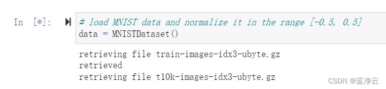
# load MNIST data and normalize it in the range [-0.5, 0.5]
data = MNISTDataset()
花的时间有亿点点久。。。真的等不下去了。。。脑子已经在修仙了。。。
看看源码写的啥
class MNISTDataset():
    def __init__(self, custom_preprocessing=None, dirpath=None):
        self._dirpath = dirpath
        if not self._dirpath:
            self._dirpath = os.path.join(os.path.dirname(os.path.abspath(__file__)),
                '..', 'data','mnist_data')

        files = ["train-images-idx3-ubyte.gz",
                 "t10k-images-idx3-ubyte.gz",
                 "train-labels-idx1-ubyte.gz",
                 "t10k-labels-idx1-ubyte.gz"]
        for name in files:
            if not os.path.exists(self._dirpath + "/" + name):
                print("retrieving file", name)
                urllib.request.urlretrieve('http://yann.lecun.com/exdb/mnist/' + name, self._dirpath + "/" + name)
                print("retrieved")

        train_data       = extract_data(self._dirpath + "/train-images-idx3-ubyte.gz", 60000)
        train_labels     = extract_labels(self._dirpath + "/train-labels-idx1-ubyte.gz", 60000)
        self.test_data   = extract_data(self._dirpath + "/t10k-images-idx3-ubyte.gz", 10000)
        self.test_labels = extract_labels(self._dirpath + "/t10k-labels-idx1-ubyte.gz", 10000)

        VALIDATION_SIZE = 5000

        self.validation_data = train_data[:VALIDATION_SIZE, :, :, :]
        self.validation_labels = train_labels[:VALIDATION_SIZE]
        self.train_data = train_data[VALIDATION_SIZE:, :, :, :]
        self.train_labels = train_labels[VALIDATION_SIZE:]
直接百度搜一下下载MNIST数据集,找到别人分享的资源,把这四个文件["train-images-idx3-ubyte.gz","t10k-images-idx3-ubyte.gz","train-labels-idx1-ubyte.gz", "t10k-labels-idx1-ubyte.gz"]下载下来。
然后代码改一下,dirpath就是那四个文件的保存路径。
dirpath = r'C:\Users\gxx\Desktop\jupter\aix360\MNIST'
data = MNISTDataset(dirpath=dirpath)
# print the shape of train and test data
print("MNIST train data range  :", "(", np.min(data.train_data), ",", np.max(data.train_data), ")")
print("MNIST test data range   :", "(", np.min(data.train_data), ",",  np.max(data.train_data), ")")
print("MNIST train data shape  :", data.train_data.shape)
print("MNIST test data shape   :", data.test_data.shape)
print("MNIST train labels shape:", data.test_labels.shape)
print("MNIST test labels shape :", data.test_labels.shape)
输出结果
MNIST train data range  : ( -0.5 , 0.5 )
MNIST test data range   : ( -0.5 , 0.5 )
MNIST train data shape  : (55000, 28, 28, 1)
MNIST test data shape   : (10000, 28, 28, 1)
MNIST train labels shape: (10000, 10)
MNIST test labels shape : (10000, 10)
加载经过训练的MNIST模型
此notebook使用经过训练的MNIST模型。此处提供了训练此模型的代码。请注意,该模型输出logits,并且不使用softmax函数。
把官网上的文件复制到本地,改一下路径。
# path to mnist related models
# model_path = '../../aix360/models/CEM'
model_path = r'C:\Users\gxx\Desktop\jupter\aix360\CEM'

def load_model(model_json_file, model_wt_file):

    # read model json file
    with open(model_json_file, 'r') as f:
        model = model_from_json(f.read())

    # read model weights file
    model.load_weights(model_wt_file)

    return model


# load MNIST model using its json and wt files
mnist_model = load_model(os.path.join(model_path, 'mnist.json'), os.path.join(model_path, 'mnist'))

# print model summary
mnist_model.summary()
不出意外,bug又来了。。。


在安装 tensorflow 时,默认安装 h5py 为3.7.0,而报错是因为安装的 TF 不支持过高版本的 h5py。
卸 载 h5py 3.7.0版本,安装 h5py 2.10.0 版本。
pip uninstall --user h5py
pip install --user h5py==2.10.0
结果输出:

加载经过训练的卷积自动编码器模型(可选)
这个notebook使用了一个经过训练的卷积自动编码器模型。此处提供了训练此模型的代码。
# load the trained convolutional autoencoder model
ae_model = load_model(os.path.join(model_path, 'mnist_AE_1_decoder.json'),
                      os.path.join(model_path, 'mnist_AE_1_decoder.h5'))
# print model summary
ae_model.summary()

初始化CEM解释程序以解释模型预测
# wrap mnist_model into a framework independent class structure
mymodel = KerasClassifier(mnist_model)

# initialize explainer object
explainer = CEMExplainer(mymodel)
解释输入实例
# choose an input image
image_id = 340
input_image = data.test_data[image_id]

# rescale values from [-0.5, 0.5] to [0, 255] for plotting
plt.imshow((input_image[:,:,0] + 0.5)*255, cmap="gray")

# check model prediction
print("Predicted class:", mymodel.predict_classes(np.expand_dims(input_image, axis=0)))
print("Predicted logits:", mymodel.predict(np.expand_dims(input_image, axis=0)))
结果输出:

观察结果:
尽管上面的图像被模型分类为数字3,但是由于它与数字5具有相似性,所以它也可以被分类为数字5。我们现在使用AIX360的CEMBexplainer来计算相关的正面和负面解释,这有助于我们理解为什么图像被模型分类为数字3而不是数字5。
获得相关否定(Pertinent Negative,PN)解释
arg_mode = "PN" # Find pertinent negative

arg_max_iter = 1000 # Maximum number of iterations to search for the optimal PN for given parameter settings
arg_init_const = 10.0 # Initial coefficient value for main loss term that encourages class change
arg_b = 9 # No. of updates to the coefficient of the main loss term

arg_kappa = 0.9 # Minimum confidence gap between the PNs (changed) class probability and original class' probability
arg_beta = 1.0 # Controls sparsity of the solution (L1 loss)
arg_gamma = 100 # Controls how much to adhere to a (optionally trained) autoencoder
arg_alpha = 0.01 # Penalizes L2 norm of the solution
arg_threshold = 0.05 # Automatically turn off features <= arg_threshold if arg_threshold < 1
arg_offset = 0.5 # the model assumes classifier trained on data normalized
                # in [-arg_offset, arg_offset] range, where arg_offset is 0 or 0.5


(adv_pn, delta_pn, info_pn) = explainer.explain_instance(np.expand_dims(input_image, axis=0), arg_mode, ae_model, arg_kappa, arg_b,
                                            arg_max_iter, arg_init_const, arg_beta, arg_gamma, arg_alpha, arg_threshold, arg_offset)
结果输出:
WARNING:tensorflow:From C:\Users\gxx\anaconda3\envs\tf-py37\lib\site-packages\aix360\algorithms\contrastive\CEM_aen.py:60: The name tf.placeholder is deprecated. Please use tf.compat.v1.placeholder instead.

WARNING:tensorflow:From C:\Users\gxx\anaconda3\envs\tf-py37\lib\site-packages\aix360\algorithms\contrastive\CEM_aen.py:151: The name tf.assign is deprecated. Please use tf.compat.v1.assign instead.

WARNING:tensorflow:From C:\Users\gxx\anaconda3\envs\tf-py37\lib\site-packages\aix360\algorithms\contrastive\CEM_aen.py:213: The name tf.train.polynomial_decay is deprecated. Please use tf.compat.v1.train.polynomial_decay instead.

WARNING:tensorflow:From C:\Users\gxx\anaconda3\envs\tf-py37\lib\site-packages\tensorflow\python\keras\optimizer_v2\learning_rate_schedule.py:409: div (from tensorflow.python.ops.math_ops) is deprecated and will be removed in a future version.
Instructions for updating:
Deprecated in favor of operator or tf.math.divide.
WARNING:tensorflow:From C:\Users\gxx\anaconda3\envs\tf-py37\lib\site-packages\aix360\algorithms\contrastive\CEM_aen.py:216: The name tf.train.GradientDescentOptimizer is deprecated. Please use tf.compat.v1.train.GradientDescentOptimizer instead.

WARNING:tensorflow:From C:\Users\gxx\anaconda3\envs\tf-py37\lib\site-packages\tensorflow\python\ops\math_grad.py:1250: add_dispatch_support.<locals>.wrapper (from tensorflow.python.ops.array_ops) is deprecated and will be removed in a future version.
Instructions for updating:
Use tf.where in 2.0, which has the same broadcast rule as np.where
WARNING:tensorflow:From C:\Users\gxx\anaconda3\envs\tf-py37\lib\site-packages\aix360\algorithms\contrastive\CEM_aen.py:230: The name tf.variables_initializer is deprecated. Please use tf.compat.v1.variables_initializer instead.

iter:0 const:[10.]
Loss_Overall:2737.2244, Loss_Attack:58.5389
Loss_L2Dist:0.0000, Loss_L1Dist:0.0000, AE_loss:2678.685546875
target_lab_score:19.3967, max_nontarget_lab_score:14.4428

iter:500 const:[10.]
Loss_Overall:2737.2244, Loss_Attack:58.5389
Loss_L2Dist:0.0000, Loss_L1Dist:0.0000, AE_loss:2678.685546875
target_lab_score:19.3967, max_nontarget_lab_score:14.4428

iter:0 const:[100.]
Loss_Overall:3152.3984, Loss_Attack:0.0000
Loss_L2Dist:12.6054, Loss_L1Dist:16.5280, AE_loss:3123.264892578125
target_lab_score:9.0004, max_nontarget_lab_score:29.0375

iter:500 const:[100.]
Loss_Overall:2977.4854, Loss_Attack:0.0000
Loss_L2Dist:7.0313, Loss_L1Dist:10.1030, AE_loss:2960.35107421875
target_lab_score:9.2486, max_nontarget_lab_score:28.5018

iter:0 const:[55.]
Loss_Overall:2840.0422, Loss_Attack:0.0000
Loss_L2Dist:4.8674, Loss_L1Dist:7.2291, AE_loss:2827.94580078125
target_lab_score:9.7374, max_nontarget_lab_score:27.1471

iter:500 const:[55.]
Loss_Overall:2670.4844, Loss_Attack:0.0000
Loss_L2Dist:0.8409, Loss_L1Dist:2.1313, AE_loss:2667.51220703125
target_lab_score:15.5937, max_nontarget_lab_score:19.4013

iter:0 const:[32.5]
Loss_Overall:2644.0203, Loss_Attack:2.0429
Loss_L2Dist:0.5595, Loss_L1Dist:1.8527, AE_loss:2639.565185546875
target_lab_score:16.7141, max_nontarget_lab_score:17.5513

iter:500 const:[32.5]
Loss_Overall:2868.9368, Loss_Attack:190.2513
Loss_L2Dist:0.0000, Loss_L1Dist:0.0000, AE_loss:2678.685546875
target_lab_score:19.3967, max_nontarget_lab_score:14.4428

iter:0 const:[21.25]
Loss_Overall:2782.8979, Loss_Attack:117.1809
Loss_L2Dist:0.0176, Loss_L1Dist:0.2093, AE_loss:2665.490234375
target_lab_score:19.1928, max_nontarget_lab_score:14.5784

iter:500 const:[21.25]
Loss_Overall:2803.0806, Loss_Attack:124.3951
Loss_L2Dist:0.0000, Loss_L1Dist:0.0000, AE_loss:2678.685546875
target_lab_score:19.3967, max_nontarget_lab_score:14.4428

iter:0 const:[26.875]
Loss_Overall:2738.9089, Loss_Attack:91.5858
Loss_L2Dist:0.1530, Loss_L1Dist:0.9359, AE_loss:2646.234130859375
target_lab_score:18.1907, max_nontarget_lab_score:15.6829

iter:500 const:[26.875]
Loss_Overall:2836.0088, Loss_Attack:157.3232
Loss_L2Dist:0.0000, Loss_L1Dist:0.0000, AE_loss:2678.685546875
target_lab_score:19.3967, max_nontarget_lab_score:14.4428

iter:0 const:[24.0625]
Loss_Overall:2774.3594, Loss_Attack:117.5742
Loss_L2Dist:0.0524, Loss_L1Dist:0.4683, AE_loss:2656.2646484375
target_lab_score:18.8622, max_nontarget_lab_score:14.8760

iter:500 const:[24.0625]
Loss_Overall:2819.5447, Loss_Attack:140.8591
Loss_L2Dist:0.0000, Loss_L1Dist:0.0000, AE_loss:2678.685546875
target_lab_score:19.3967, max_nontarget_lab_score:14.4428

iter:0 const:[25.46875]
Loss_Overall:2754.6963, Loss_Attack:104.3005
Loss_L2Dist:0.0950, Loss_L1Dist:0.7232, AE_loss:2649.57763671875
target_lab_score:18.5058, max_nontarget_lab_score:15.3106

iter:500 const:[25.46875]
Loss_Overall:2827.7766, Loss_Attack:149.0911
Loss_L2Dist:0.0000, Loss_L1Dist:0.0000, AE_loss:2678.685546875
target_lab_score:19.3967, max_nontarget_lab_score:14.4428

iter:0 const:[24.765625]
Loss_Overall:2762.2129, Loss_Attack:109.3322
Loss_L2Dist:0.0725, Loss_L1Dist:0.6168, AE_loss:2652.191650390625
target_lab_score:18.6550, max_nontarget_lab_score:15.1403

iter:500 const:[24.765625]
Loss_Overall:2823.6606, Loss_Attack:144.9751
Loss_L2Dist:0.0000, Loss_L1Dist:0.0000, AE_loss:2678.685546875
target_lab_score:19.3967, max_nontarget_lab_score:14.4428
print(info_pn)
结果输出:
[INFO]kappa:0.9, Orig class:3, Perturbed class:5, Delta class: 1, Orig prob:[[-11.279339 0.73625 -9.008647 19.396711 -8.286123 14.442826 -1.3170443 -11.587322 -0.992185 1.0182207]], Perturbed prob:[[ -6.6607647 -1.9869652 -7.4231925 13.461045 -6.341817 13.8300295 1.2803447 -11.60892 0.31489015 1.1112802 ]], Delta prob:[[-0.11039171 1.0537697 -0.0954444 -0.2623107 -0.3357536 0.24241148 -0.0948096 -0.00691785 -0.31975082 -0.56200165]]
获得相关的肯定(Pertinent Positive,PP)解释
arg_mode = "PP"  # Find pertinent positive
arg_beta = 0.1 # Controls sparsity of the solution (L1 loss)
(adv_pp, delta_pp, info_pp) = explainer.explain_instance(np.expand_dims(input_image, axis=0), arg_mode, ae_model, arg_kappa, arg_b,
                                            arg_max_iter, arg_init_const, arg_beta, arg_gamma, arg_alpha, arg_threshold, arg_offset)
结果输出:
iter:0 const:[10.]
Loss_Overall:1186.7114, Loss_Attack:20.4772
Loss_L2Dist:0.0000, Loss_L1Dist:0.0000, AE_loss:1166.2342529296875
target_lab_score:-0.1036, max_nontarget_lab_score:1.0441

iter:500 const:[10.]
Loss_Overall:1186.7114, Loss_Attack:20.4772
Loss_L2Dist:0.0000, Loss_L1Dist:0.0000, AE_loss:1166.2342529296875
target_lab_score:-0.1036, max_nontarget_lab_score:1.0441

iter:0 const:[100.]
Loss_Overall:1374.8175, Loss_Attack:224.8764
Loss_L2Dist:0.0581, Loss_L1Dist:0.5667, AE_loss:1149.8262939453125
target_lab_score:-0.1908, max_nontarget_lab_score:1.1579

iter:500 const:[100.]
Loss_Overall:1177.7847, Loss_Attack:0.0000
Loss_L2Dist:9.0615, Loss_L1Dist:26.9499, AE_loss:1166.0281982421875
target_lab_score:9.1723, max_nontarget_lab_score:5.3354

iter:0 const:[55.]
Loss_Overall:1278.8588, Loss_Attack:112.6245
Loss_L2Dist:0.0000, Loss_L1Dist:0.0000, AE_loss:1166.2342529296875
target_lab_score:-0.1036, max_nontarget_lab_score:1.0441

iter:500 const:[55.]
Loss_Overall:1278.8588, Loss_Attack:112.6245
Loss_L2Dist:0.0000, Loss_L1Dist:0.0000, AE_loss:1166.2342529296875
target_lab_score:-0.1036, max_nontarget_lab_score:1.0441

iter:0 const:[77.5]
Loss_Overall:1324.9324, Loss_Attack:158.6981
Loss_L2Dist:0.0000, Loss_L1Dist:0.0000, AE_loss:1166.2342529296875
target_lab_score:-0.1036, max_nontarget_lab_score:1.0441

iter:500 const:[77.5]
Loss_Overall:1324.9324, Loss_Attack:158.6981
Loss_L2Dist:0.0000, Loss_L1Dist:0.0000, AE_loss:1166.2342529296875
target_lab_score:-0.1036, max_nontarget_lab_score:1.0441

iter:0 const:[88.75]
Loss_Overall:1347.3350, Loss_Attack:190.4548
Loss_L2Dist:0.0195, Loss_L1Dist:0.2384, AE_loss:1156.8367919921875
target_lab_score:-0.1378, max_nontarget_lab_score:1.1082

iter:500 const:[88.75]
Loss_Overall:1182.4167, Loss_Attack:0.0000
Loss_L2Dist:10.1261, Loss_L1Dist:29.5733, AE_loss:1169.3333740234375
target_lab_score:10.9503, max_nontarget_lab_score:8.5652

iter:0 const:[83.125]
Loss_Overall:1336.9946, Loss_Attack:176.8078
Loss_L2Dist:0.0096, Loss_L1Dist:0.1385, AE_loss:1160.1634521484375
target_lab_score:-0.1352, max_nontarget_lab_score:1.0918

iter:500 const:[83.125]
Loss_Overall:1177.7847, Loss_Attack:0.0000
Loss_L2Dist:9.0615, Loss_L1Dist:26.9499, AE_loss:1166.0281982421875
target_lab_score:9.1723, max_nontarget_lab_score:5.3355

iter:0 const:[80.3125]
Loss_Overall:1330.7108, Loss_Attack:169.8772
Loss_L2Dist:0.0070, Loss_L1Dist:0.1182, AE_loss:1160.8148193359375
target_lab_score:-0.1306, max_nontarget_lab_score:1.0846

iter:500 const:[80.3125]
Loss_Overall:1187.8037, Loss_Attack:0.0000
Loss_L2Dist:9.0935, Loss_L1Dist:26.5365, AE_loss:1176.0565185546875
target_lab_score:10.0619, max_nontarget_lab_score:2.9340

iter:0 const:[78.90625]
Loss_Overall:1327.5865, Loss_Attack:166.4040
Loss_L2Dist:0.0058, Loss_L1Dist:0.1080, AE_loss:1161.1658935546875
target_lab_score:-0.1282, max_nontarget_lab_score:1.0807

iter:500 const:[78.90625]
Loss_Overall:1176.6401, Loss_Attack:0.0000
Loss_L2Dist:8.3147, Loss_L1Dist:24.4263, AE_loss:1165.8828125
target_lab_score:8.1241, max_nontarget_lab_score:4.7113

iter:0 const:[78.203125]
Loss_Overall:1326.0416, Loss_Attack:164.6752
Loss_L2Dist:0.0053, Loss_L1Dist:0.1030, AE_loss:1161.350830078125
target_lab_score:-0.1270, max_nontarget_lab_score:1.0788

iter:500 const:[78.203125]
Loss_Overall:1180.0135, Loss_Attack:0.0000
Loss_L2Dist:9.0324, Loss_L1Dist:26.5381, AE_loss:1168.327392578125
target_lab_score:9.0967, max_nontarget_lab_score:5.0136
print(info_pp)
结果输出:
[INFO]kappa:0.9, Orig class:3, Perturbed class:3, Delta class: 3, Orig prob:[[-11.279339 0.73625 -9.008647 19.396711 -8.286123 14.442826 -1.3170443 -11.587322 -0.992185 1.0182207]], Perturbed prob:[[ -6.0453925 -0.16173983 -6.025815 11.575153 -3.0273986 11.318211 4.259432 -11.328725 -1.0278873 -2.3766122 ]], Delta prob:[[-2.3122752 0.60199463 -0.6148693 4.709517 -2.2623286 1.0073487 -2.2190797 -0.83646446 -1.5357832 0.9802128 ]]
相关负(PN)和相关正(PP)解释图
# rescale values from [-0.5, 0.5] to [0, 255] for plotting
fig0 = (input_image[:,:,0] + 0.5)*255

fig1 = (adv_pn[0,:,:,0] + 0.5) * 255
fig2 = (fig1 - fig0) #rescaled delta_pn
fig3 = (adv_pp[0,:,:,0] + 0.5) * 255
fig4 = (delta_pp[0,:,:,0] + 0.5) * 255 #rescaled delta_pp

f, axarr = plt.subplots(1, 5, figsize=(10,10))
axarr[0].set_title("Original" + "(" + str(mymodel.predict_classes(np.expand_dims(input_image, axis=0))[0]) + ")")
axarr[1].set_title("Original + PN" + "(" + str(mymodel.predict_classes(adv_pn)[0]) + ")")
axarr[2].set_title("PN")
axarr[3].set_title("Original + PP")
axarr[4].set_title("PP" + "(" + str(mymodel.predict_classes(delta_pp)[0]) + ")")

axarr[0].imshow(fig0, cmap="gray")
axarr[1].imshow(fig1, cmap="gray")
axarr[2].imshow(fig2, cmap="gray")
axarr[3].imshow(fig3, cmap="gray")
axarr[4].imshow(fig4, cmap="gray")
plt.show()
结果输出:
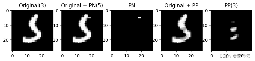
说明:
- PP突出显示图像中存在的最小像素集,以便将其分类为数字3。注意,原始图像和PP都被分类器分类为数字3。
- PN在顶部突出显示一条小水平线,该水平线的存在会将原始图像的分类改变为数字5,因此应该不存在,以便分类保持为数字3。


 被折叠的 条评论
为什么被折叠?
被折叠的 条评论
为什么被折叠?
 到【灌水乐园】发言


