分别用最小二乘法和梯度下降法实现线性回归

下面代码中包含了两种方法

import numpy as np

np.random.seed(1234)

x = np.random.rand(500, 3)
# x为数据，500个样本，每个样本三个自变量
y = x.dot(np.array([4.2, 5.7, 10.8]))
# y为标签，每个样本对应一个y值

# 最小二乘法
class LR_LS():
    def __init__(self):
        self.w = None

    def fit(self, X, y):
        self.w = np.linalg.inv(X.T.dot(X)).dot(X.T).dot(y)

    def predict(self, X):
        y_pred = X.dot(self.w)

        return y_pred

# 梯度下降法
class LR_GradientDescent():
    def __init__(self):
        self.w = None
        self.cnt = 0

    def fit(self, X, y, alpha = 0.02, loss = 1e-10):
        y = y.reshape(-1, 1)
        [m, d] = np.shape(X)
        self.w = np.zeros(d)
        tol = 1e5

        while tol > loss:
            h_f = X.dot(self.w).reshape(-1, 1)
            theta = self.w + alpha * np.mean(X * (y - h_f), axis = 0)
            tol = np.sum(np.abs(theta - self.w))
            self.w = theta
            self.cnt += 1

    def predict(self, X):
        return X.dot(self.w)


if __name__ == '__main__':
    lr_ls = LR_LS()
    lr_ls.fit(x, y)
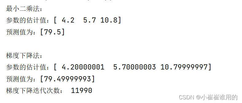
    print("最小二乘法：")
    print("参数的估计值：%s" %(lr_ls.w))

    x_test = np.array([2, 3, 5]).reshape(1, -1)
    print("预测值为：%s" %(lr_ls.predict(x_test)))
    print()

    lr_gd = LR_GradientDescent()
    lr_gd.fit(x, y)
    print("梯度下降法：")
    print("参数的估计值：%s" % (lr_gd.w))

    x_test = np.array([2, 3, 5]).reshape(1, -1)
    print("预测值为：%s" % (lr_gd.predict(x_test)))
    print("梯度下降迭代次数：", lr_gd.cnt)

运行结果为：