


一、数据
https://github.com/CynicallyAcclaimed/University-Admissions-Predictor/tree/main
以下为机翻:
大学录取预测器
根据前几年的录取统计数据,建立一个可以预测大学录取情况的模型。
作为我为申请HCI课程研究生课程的学生设计的应用程序的一部分(工作正在进行中),我正在构建一个简单的预测器,可以预测学生被特定大学录取的机会。这是根据前几年申请的学生的统计数据得出的。我通过Yocket、GradCafe和某个众包谷歌数据表收集了这些数据。
由于人机交互仍然是一个不断发展的领域,关于它的数据并不多。我设法获得了大约250张唱片,分布在不同的大学。虽然应用程序的目的是随着时间的推移生成更多的数据,允许模型迭代学习,但目前还不够。因此,为了改进模型,我研究了基于现有集合综合生成更多数据的方法。
我已经探索了不同类型的GAN模型,对于我的目的来说,CTGAN是最好的方法。我们比较了不同模型和数据点数量下的准确率,每所大学的平均准确率达到75%。
数据表信息:
GRE和托福成绩可以是NA,因为:(a)大学不要求成绩;(b)学生有豁免或不需要提交成绩
CGPA为均匀性转换为4.0刻度
根据GradCafe的批注,学生身份:国际学生I;国内学生A级;具有国内本科学位的国际学生
QS和泰晤士高等教育的排名从2020年开始,可能会有所变化
二、参考文章
【Python深度学习系列】十几行代码教你使用CTGAN模拟生成表格数据_hci-data-优快云博客
三、代码及解析
import pandas as pd
import numpy as np
from sklearn import preprocessing
from ctgan import CTGAN
import ctgan
# ctgan版本0.5.0中是有ctgan.evaluation的,但我安装的0.10.2,已经没有这个模块了,后续用统计方法来评估
from scipy import stats
import matplotlib.pyplot as plt
# 准备原始数据
hci_data=pd.read_csv(r'HCI_Datasheet.csv')
hci_data=hci_data.drop(columns=['S. No','Decision Date','Application Date'])
# 创建了一个新的列 'University_Program',其值是 'University' 列和 'Programme' 列的值用空格连接起来的结果
hci_data['University_Program']=hci_data.University+' '+hci_data.Programme
hci_data.University=hci_data.University_Program
hci_data=hci_data.drop(columns=['Programme','University_Program','Year of Entry'])
print("增删列后的数据",hci_data)
# LabelEncoder 是 sklearn.preprocessing 模块中的一个工具类,
# 主要用于将分类变量(即文本形式的类别标签)转换为数值形式的标签。
le = preprocessing.LabelEncoder()
# fit_transform 是 LabelEncoder 对象的一个方法,它实际上是 fit 方法和 transform 方法的组合
# fit 方法会遍历输入的分类变量的所有值,收集其中不同的类别,从 0 开始,为每个类别分配一个唯一的整数编码。
# transform 方法会根据 fit 阶段分配的编码,将输入的分类变量中的每个类别替换为对应的整数编码。
# 例如'Rejected' 被分配了编码 1,那么 transform 方法会将 hci_data['Decision'] 列中的所有所有 'Rejected' 替换为 1
# 早期的fit_transform是先读取到哪个类别,哪个类别的标签就是0
# 但现在的fit_transform通常是按照字母顺序对类别进行编码
hci_data['Decision'] = le.fit_transform(hci_data['Decision']) ### 1-Accepted, 0-Rejected
hci_data['Research Experience'] = le.fit_transform(hci_data['Research Experience'])
hci_data['Submitted Portfolio'] = le.fit_transform(hci_data['Submitted Portfolio'])
hci_data['Student Status'] = le.fit_transform(hci_data['Student Status'])
# fillna 方法将缺失值替换为指定的值
hci_data['GRE']=hci_data['GRE'].fillna(330)
hci_data['TOEFL']=hci_data['TOEFL'].fillna(120)
print("转化类别标签及替换缺失值后的数据",hci_data)
columns=list(hci_data.columns)
print("列名为:", columns)
# 识别离散列
discrete_columns = ['University', 'Decision', 'Work Experience',\
'Research Experience', 'Submitted Portfolio', 'Student Status']
# 创建 CTGAN 对象
ctgan = CTGAN(epochs=100)
# 拟合数据,指定离散列
ctgan.fit(hci_data, discrete_columns=discrete_columns)
# 生成模拟数据
synthetic_data = ctgan.sample(len(hci_data))
print("生成的数据",synthetic_data)
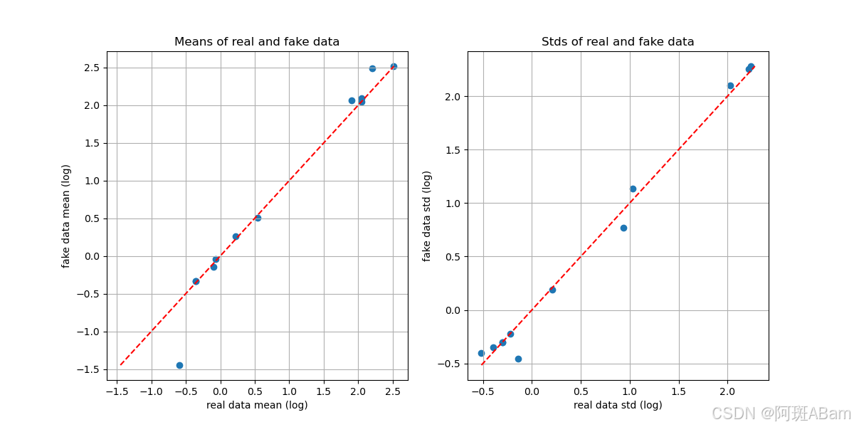
# 效果评价
# 计算均值的对数
real_mean_log = np.log10(hci_numeric.mean())
fake_mean_log = np.log10(synthetic_numeric.mean())
# 计算标准差的对数
real_std_log = np.log10(hci_numeric.std())
fake_std_log = np.log10(synthetic_numeric.std())
# 绘制均值的对数散点图
plt.figure(figsize=(12, 6))
plt.subplot(1, 2, 1)
plt.scatter(real_mean_log, fake_mean_log)
plt.plot([np.min([real_mean_log.min(), fake_mean_log.min()]), np.max([real_mean_log.max(), fake_mean_log.max()])],
[np.min([real_mean_log.min(), fake_mean_log.min()]), np.max([real_mean_log.max(), fake_mean_log.max()])], 'r--')
plt.xlabel('real data mean (log)')
plt.ylabel('fake data mean (log)')
plt.title('Means of real and fake data')
plt.grid(True)
# 绘制标准差的对数散点图
plt.subplot(1, 2, 2)
plt.scatter(real_std_log, fake_std_log)
plt.plot([np.min([real_std_log.min(), fake_std_log.min()]), np.max([real_std_log.max(), fake_std_log.max()])],
[np.min([real_std_log.min(), fake_std_log.min()]), np.max([real_std_log.max(), fake_std_log.max()])], 'r--')
plt.xlabel('real data std (log)')
plt.ylabel('fake data std (log)')
plt.title('Stds of real and fake data')
plt.grid(True)
plt.savefig('Means and Stds of real and fake data.png')
# 绘制每个特征的分布柱状图
num_plots = hci_numeric.shape[1]
num_cols = 3
num_rows = int(np.ceil(num_plots / num_cols))
plt.figure(figsize=(12, 3 * num_rows))
for i, col in enumerate(hci_numeric.columns):
plt.subplot(num_rows, num_cols, i + 1)
hci_numeric[col].hist(alpha=0.5, label='real', bins=20)
synthetic_numeric[col].hist(alpha=0.5, label='fake', bins=20)
plt.xlabel(col)
plt.ylabel('Frequency')
plt.title(f'Distribution of {col}')
plt.legend()
plt.tight_layout()
plt.savefig(f'Distribution')四、输出
增删列后的数据                University  Decision  CGPA    GRE  TOEFL  ...  Submitted Portfolio Student Status  Class Size THE Rank QS Rank
0     Georgia Tech MS HCI  Rejected  3.80    NaN  117.0  ...                  Yes              I          52       38      70
1     Georgia Tech MS HCI  Rejected  3.50    NaN  112.0  ...                  Yes              I          52       38      70
2     Georgia Tech MS HCI  Rejected  3.20    NaN    NaN  ...                  Yes              A          52       38      70
3     Georgia Tech MS HCI  Rejected  2.70  320.0  113.0  ...                  Yes              I          52       38      70
4     Georgia Tech MS HCI  Rejected  3.60  320.0    NaN  ...                  Yes              U          52       38      70
..                    ...       ...   ...    ...    ...  ...                  ...            ...         ...      ...     ...
247  Carnegie Mellon MHCI  Accepted  3.92  322.0    NaN  ...                  Yes              A          60       28      51
248  Carnegie Mellon MHCI  Accepted  3.70  324.0    NaN  ...                  Yes              U          60       28      51
249  Carnegie Mellon MHCI  Accepted  3.80  320.0    NaN  ...                  Yes              A          60       28      51
250  Carnegie Mellon MHCI  Accepted  3.80  325.0    NaN  ...                  Yes              A          60       28      51
251  Carnegie Mellon MHCI  Accepted  3.60  318.0    NaN  ...                  Yes              A          60       28      51

[252 rows x 13 columns]


转化类别标签及替换缺失值后的数据                University  Decision  CGPA    GRE  TOEFL  ...  Submitted Portfolio  Student Status  Class Size  THE Rank  QS Rank
0     Georgia Tech MS HCI         1  3.80  330.0  117.0  ...                    1               1          52        38       70
1     Georgia Tech MS HCI         1  3.50  330.0  112.0  ...                    1               1          52        38       70
2     Georgia Tech MS HCI         1  3.20  330.0  120.0  ...                    1               0          52        38       70
3     Georgia Tech MS HCI         1  2.70  320.0  113.0  ...                    1               1          52        38       70
4     Georgia Tech MS HCI         1  3.60  320.0  120.0  ...                    1               2          52        38       70
..                    ...       ...   ...    ...    ...  ...                  ...             ...         ...       ...      ...
247  Carnegie Mellon MHCI         0  3.92  322.0  120.0  ...                    1               0          60        28       51
248  Carnegie Mellon MHCI         0  3.70  324.0  120.0  ...                    1               2          60        28       51
249  Carnegie Mellon MHCI         0  3.80  320.0  120.0  ...                    1               0          60        28       51
250  Carnegie Mellon MHCI         0  3.80  325.0  120.0  ...                    1               0          60        28       51
251  Carnegie Mellon MHCI         0  3.60  318.0  120.0  ...                    1               0          60        28       51

[252 rows x 13 columns]


列名为: ['University', 'Decision', 'CGPA', 'GRE', 'TOEFL', 'Work Experience', 'Research Experience', 'Research Papers', 'Submitted Portfolio', 'Student Status', 'Class Size', 'THE Rank', 'QS Rank']


生成的数据                            University  Decision      CGPA         GRE  ...  Student Status  Class Size  THE Rank  QS Rank
0      University of Washington MHCID         1  4.116536  311.717452  ...               1          44        57      531
1          University of Michigan MSI         1  3.896665  329.220923  ...               1          46       162      200
2    University of Washington MS HCDE         0  3.897515  283.763623  ...               1          32        31      255
3                 Georgia Tech MS HCI         0  3.614945  310.372142  ...               1          61       446      487
4    Indiana University Purdue MS HCI         0  3.787183  313.147494  ...               1          36         6      578
..                                ...       ...       ...         ...  ...             ...         ...       ...      ...
247  University of Washington MS HCDE         1  3.890691  320.100153  ...               0          82        -5      180
248    University of Washington MHCID         1  3.856594  313.092709  ...               1          84        56      110
249  University of Washington MS HCDE         0  2.610085  305.625586  ...               0          83         1      172
250    University of Washington MHCID         1  3.886925  316.462298  ...               0          80        34      518
251   University of Texas Austin MSIS         0  4.037605  327.281358  ...               0          61        -9      184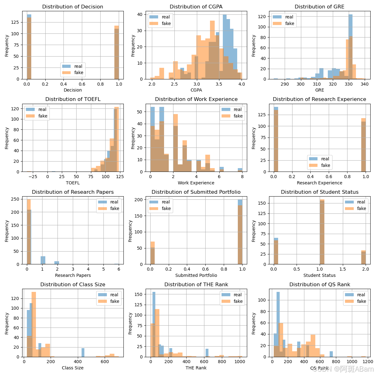


 被折叠的 条评论
为什么被折叠?
被折叠的 条评论
为什么被折叠?
 到【灌水乐园】发言


