Data Mining2复习笔记4 - Neural Networks and Deep Learning

4. Neural Networks and Deep Learning

4.1 Recap of neural networks

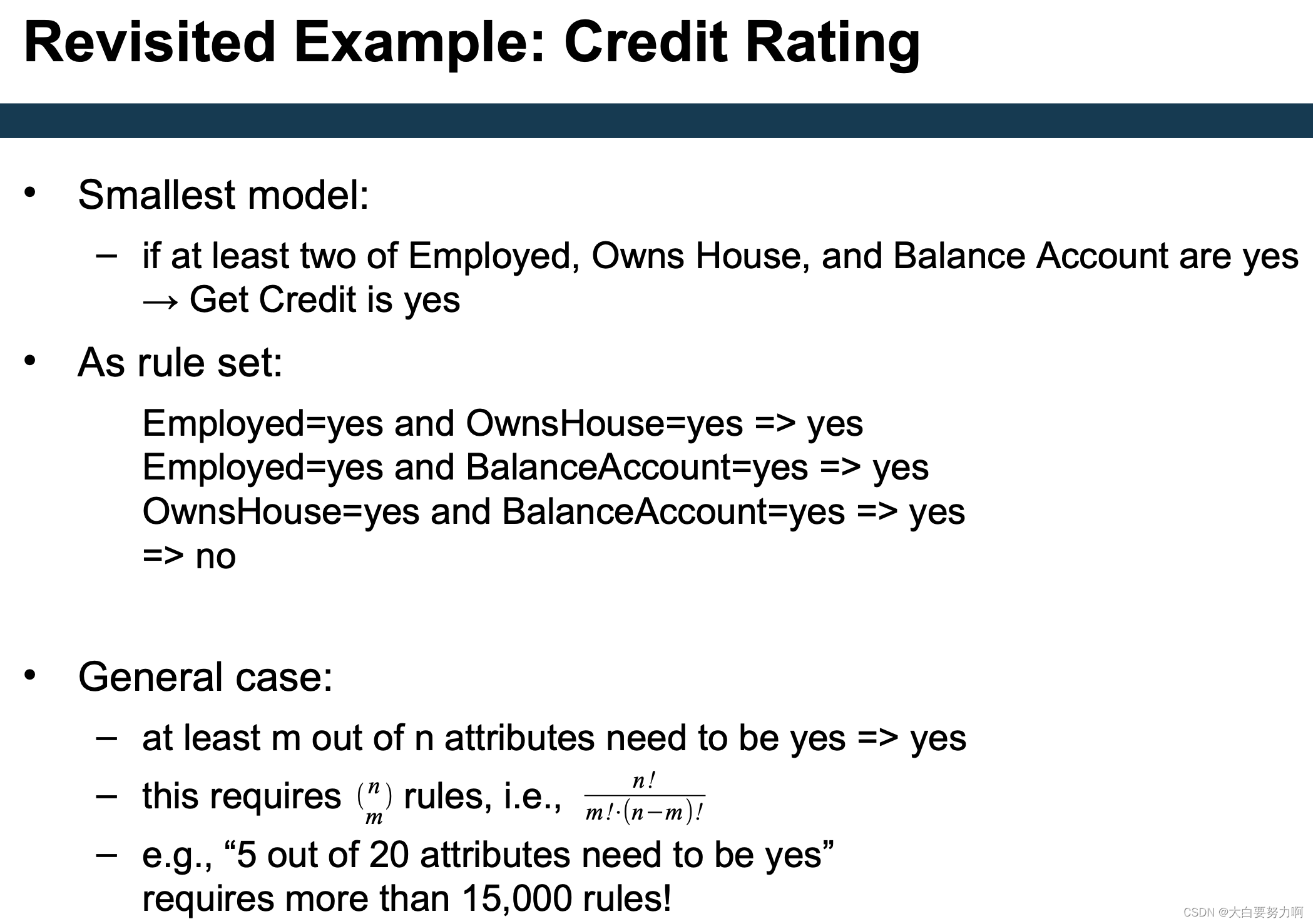
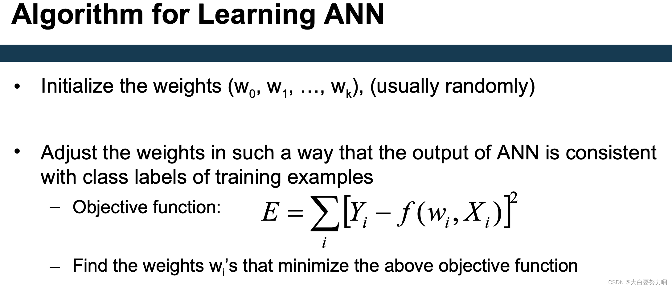
Smallest model: if at least two of Employed, Owns House, and Balance Account are yes → Get Credit is yes
Given that we represent yes and no by 1 and 0, we want if(Employed + Owns House + Balance Acount)>1.5 → Get Credit is yes

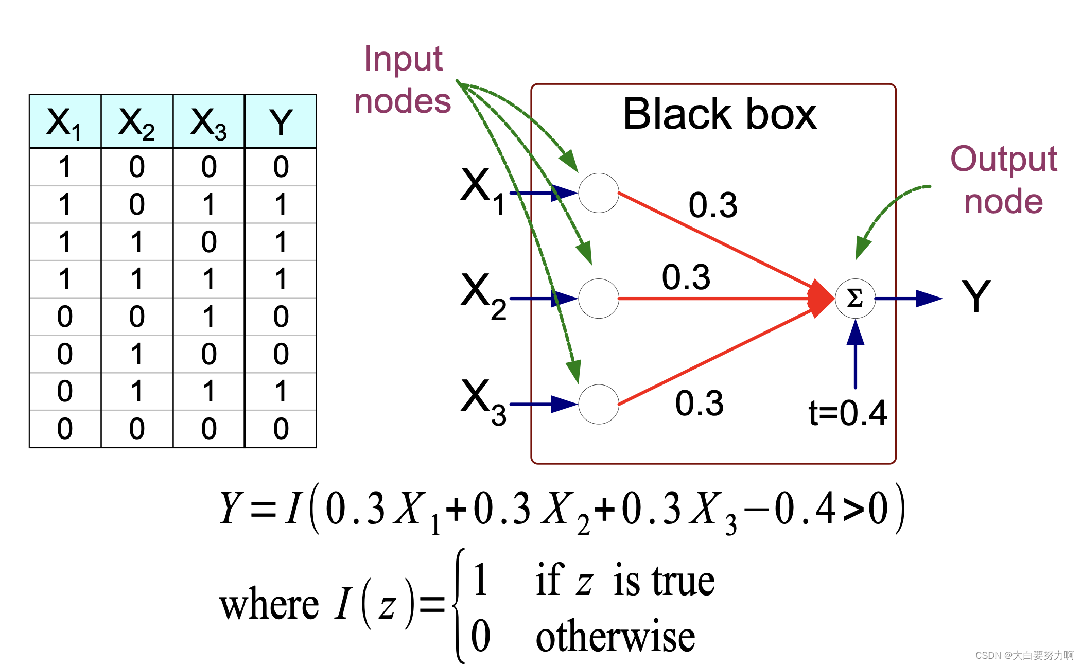
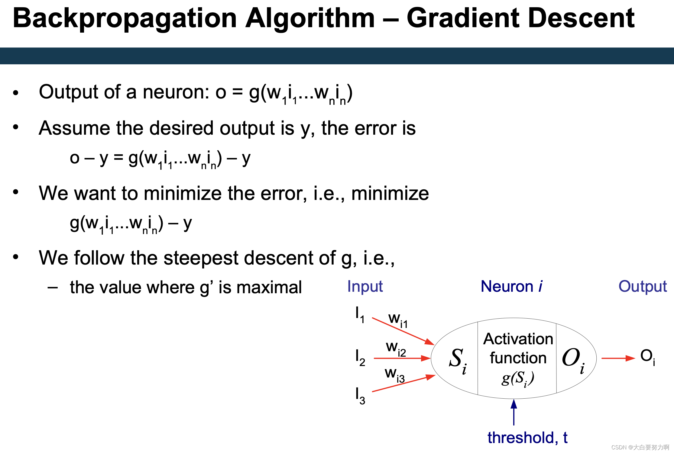
Model is an assembly of inter-connected nodes and weighted links
Output node sums up each of its input value according to the weights of its links
Compare output node against some threshold t

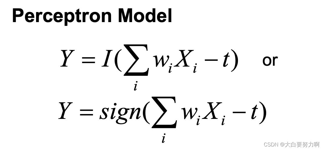
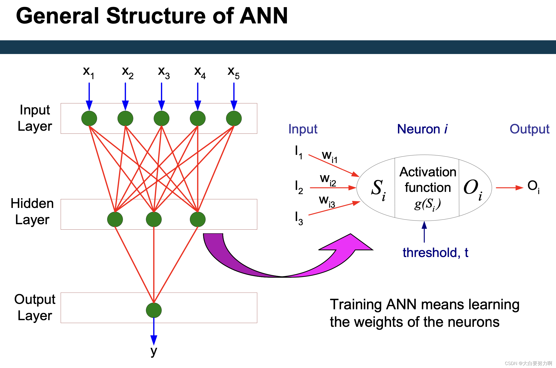
This is simple for a single layer perceptron. But for a multi-layer network, Yi is not known.

4.2 The backpropagation algorithm

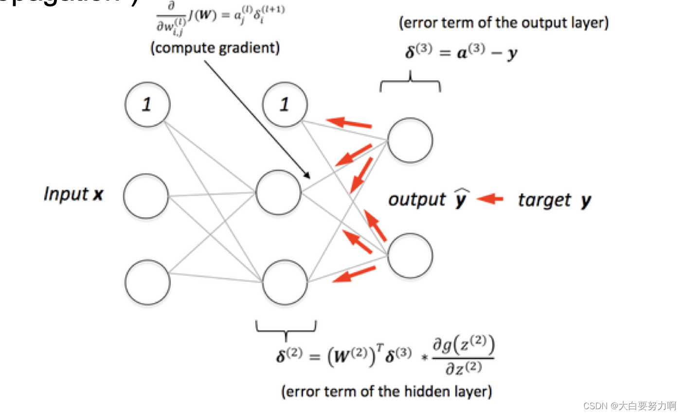
Sketch of the Backpropagation Algorithm

1. Present an example to the ANN
2. Compute error at the output layer
3. Distribute error to hidden layer according to weights
   i.e., the error is distributed according to the contribution of the previous neurons to the result
4. Adjust weights so that the error is minimized
   Adjustment factor: learning rate
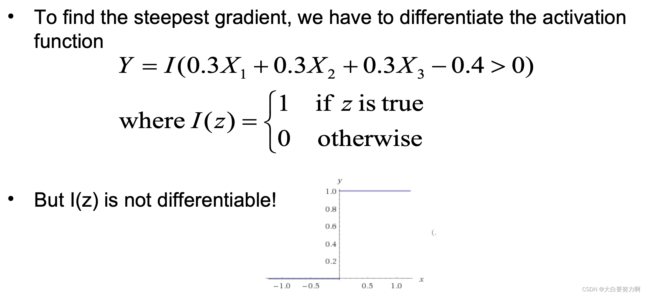
   Use gradient descent
5. Repeat until input layer is reached

4.2.1 Training in Batches

In theory, one could present the examples one after the other
In practice: use batches

• Neural network gets to see a number of examples (batch)
• All examples in the batch are predicted by the network
• Errors are accumulated
• Weights in the neural network are adapted (backpropagated) after predicting all examples in the batch

Pros: fewer model updates, faster convergence
Cons: may not find global optimum, harder to handle imbalanced datasets

4.2.2 Backpropagation Algorithm

Important notions:
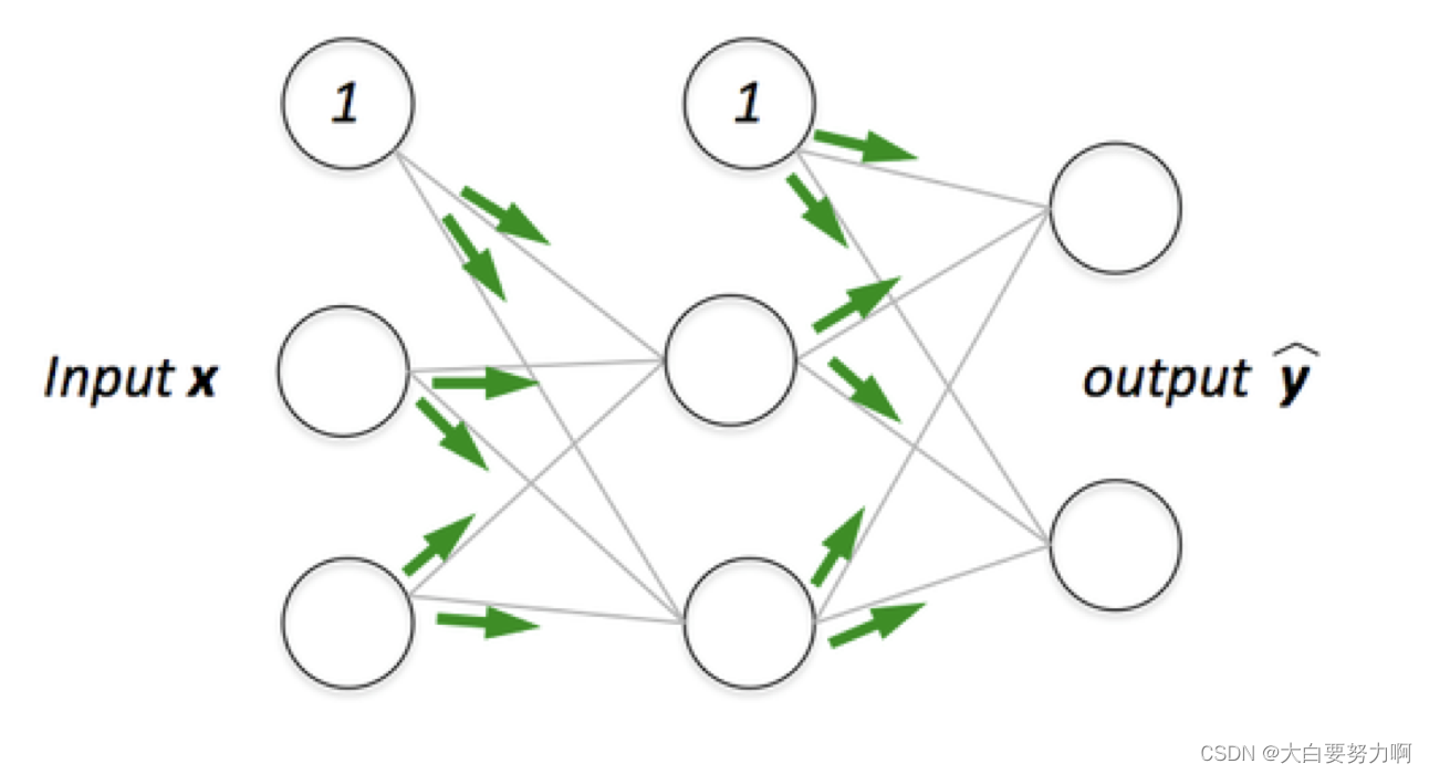
Predictions are pushed forward through the network (“feed-forward neural network”)
Errors are pushed backwards through the network (“backpropagation”)

Properties of ANNs and Backpropagation
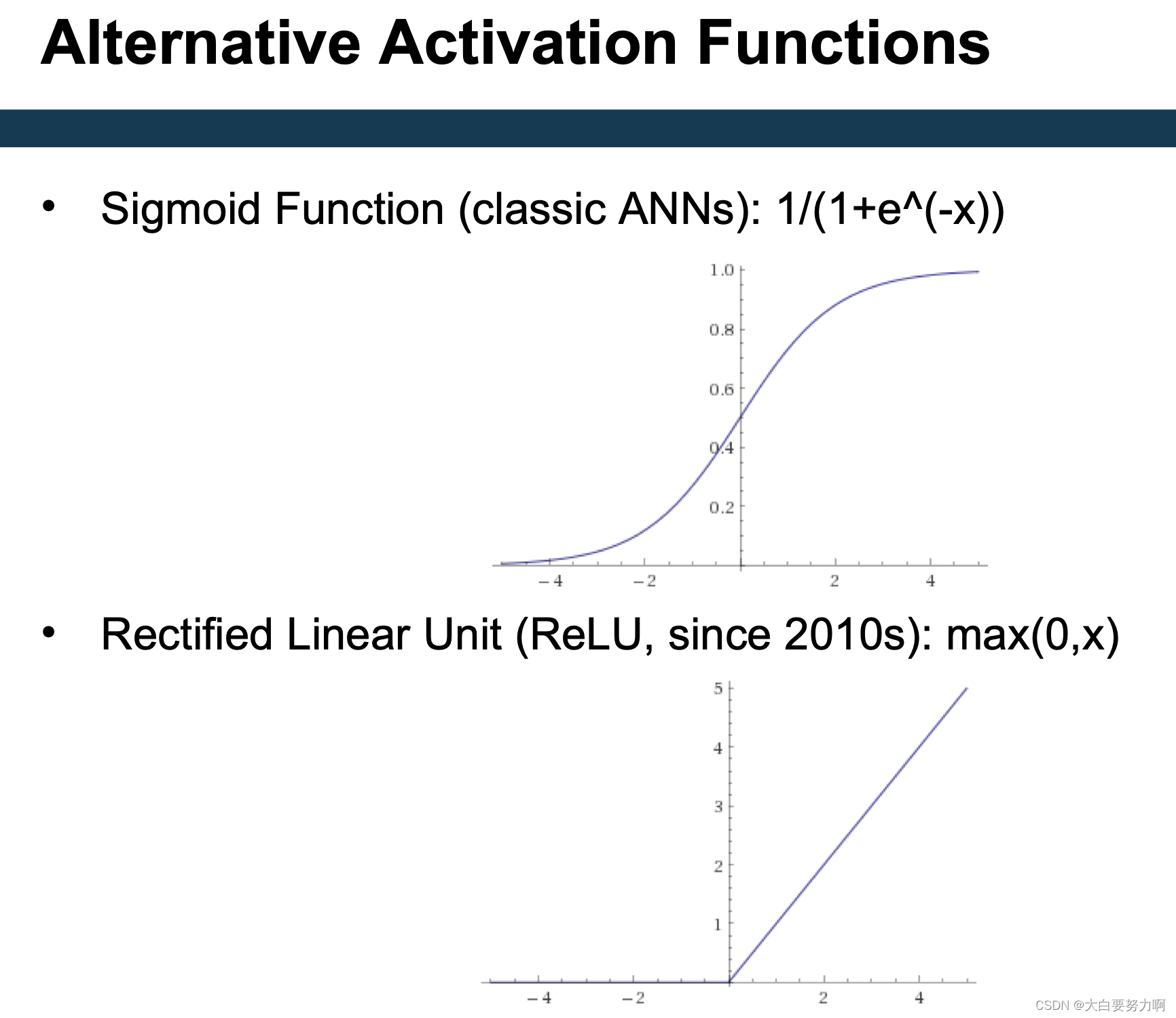
Non-linear activation function: May approximate any arbitrary function, even with one hidden layer

Convergence
Convergence may take time & higher learning rate, faster convergence

Gradient Descent Strategy
Danger of ending in local optima: Use momentum to prevent getting stuck
Lower learning rate, higher probability of finding global optimum

4.2.3 Learning Rate, Momentum, and Local Minima

Learning rate: how much do we adapt the weights with each step
0: no adaptation, use previous weight
1: forget everything we have learned so far, simply use weights that are best for current example

Smaller: slow convergence, less overfitting
Higher: faster convergence, more overfitting

---

Momentum: how much do we change the adaptation of weights
Small: allow changes in every direction soon
High: keep changing in the same direction for longer

Smaller: better convergence, sticks in local minimum
Higher: worse convergence, does not get stuck

Local Learning Rates
Observation: not all parameters change equally often, e.g., text classification: input neuron weights for infrequent words

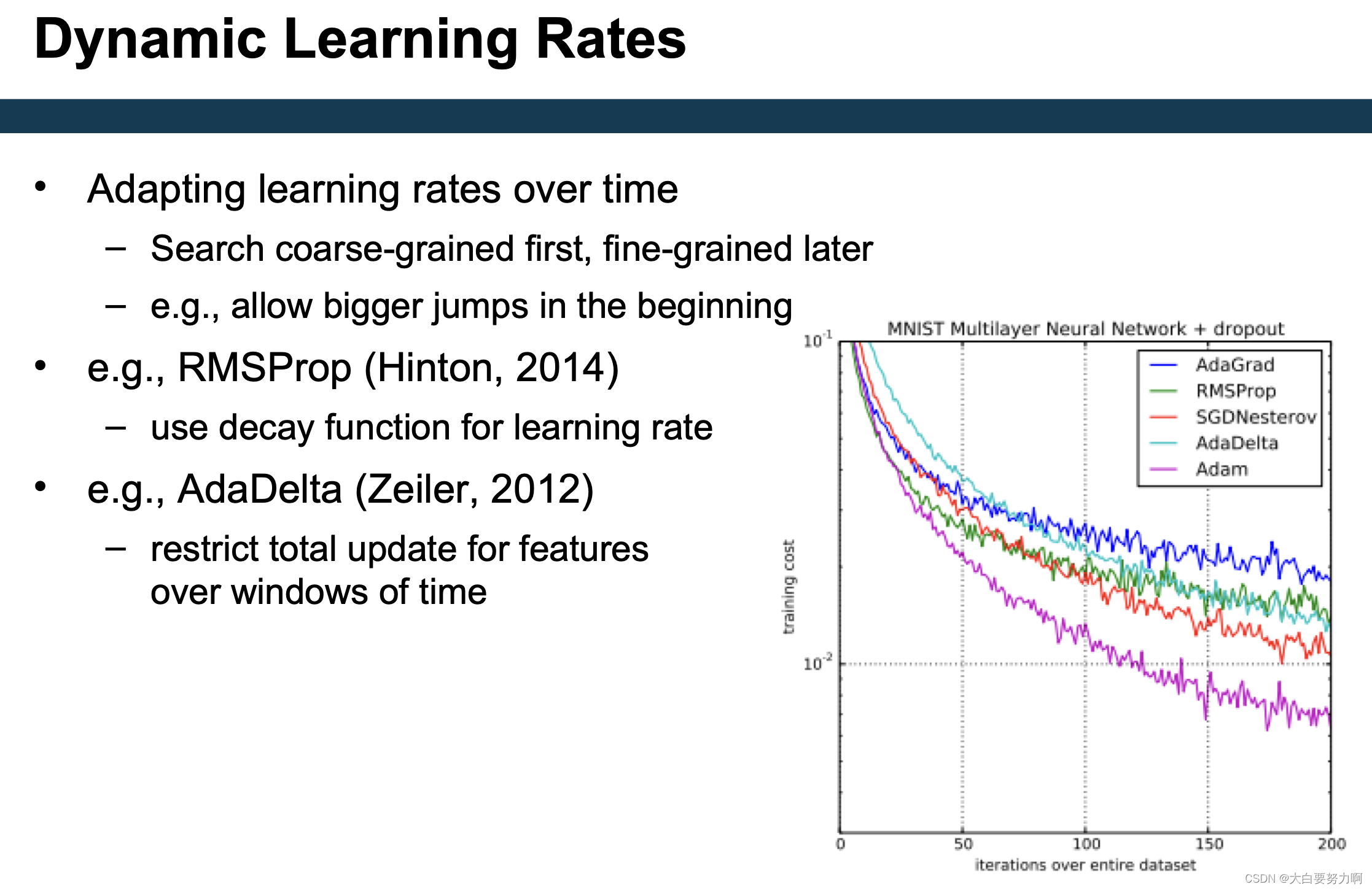
AdaGrad (Duchi et al., 2011)
maintain list of gradient changes for each parameter
adapt learning rates locally

AdaDelta (Zeiler, 2012)
restrict total updates per parameter

Bottom line: optimization functions often have a large impact.
Optimization functions are used to adjust the parameters of a neural network to minimize (or maximize) a defined loss function. The objective of optimization functions is to find parameter values that minimize (or maximize) the loss function.

ANNs vs. SVMs
ANNs have arbitrary decision boundaries – and keep the data as it is
SVMs have linear decision boundaries – and transform the data first

Recap: Feature Subset Selection & PCA
Idea: reduce the dimensionality of high dimensional data
Feature Subset Selection: focus on relevant attributes
PCA: create new attributes

In both cases
We assume that the data can be described with fewer variables
Without losing much information

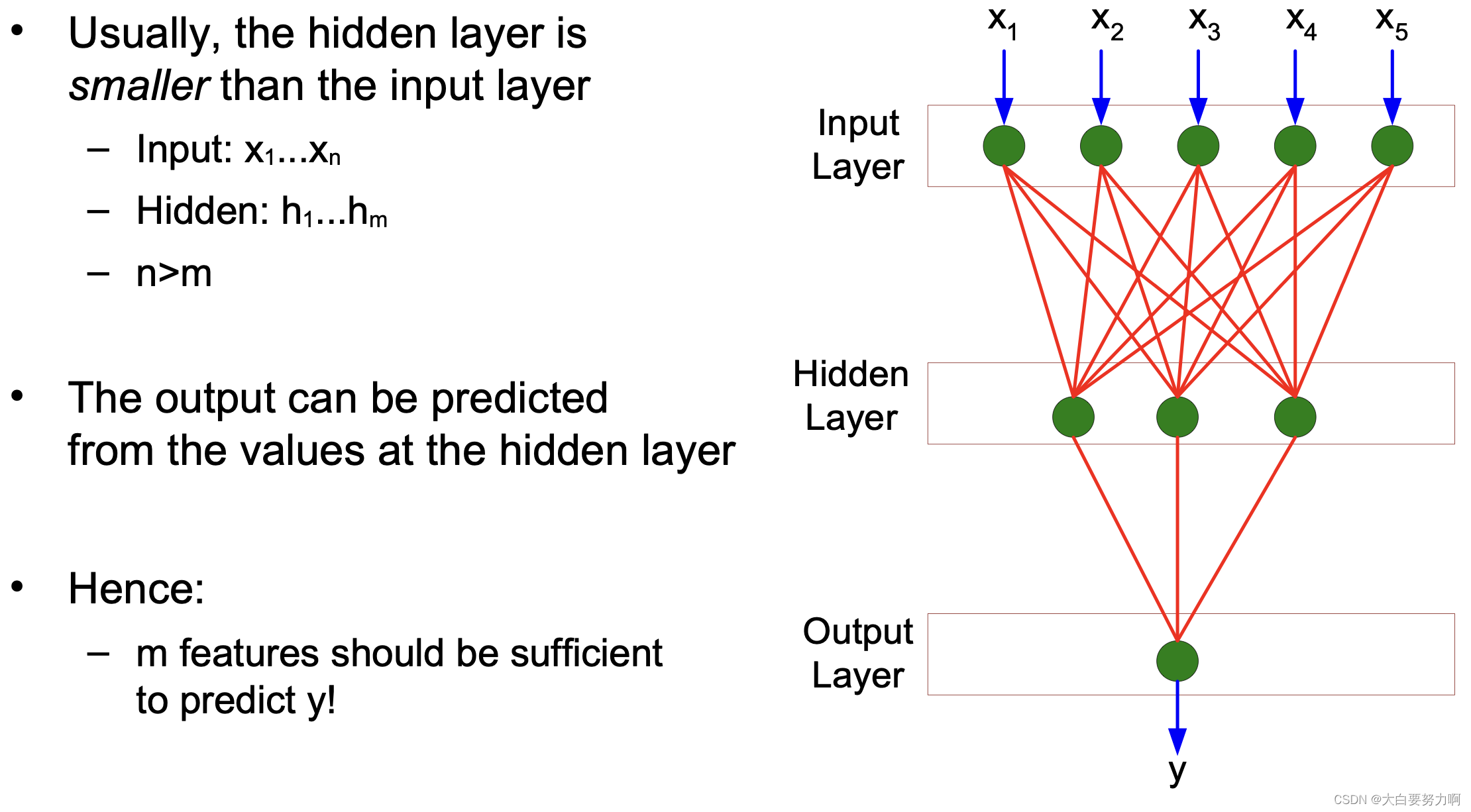
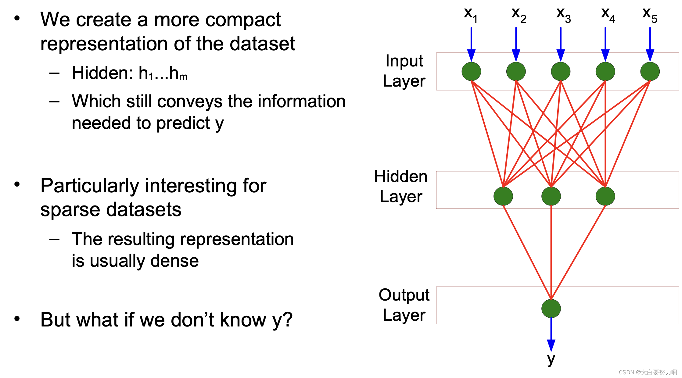
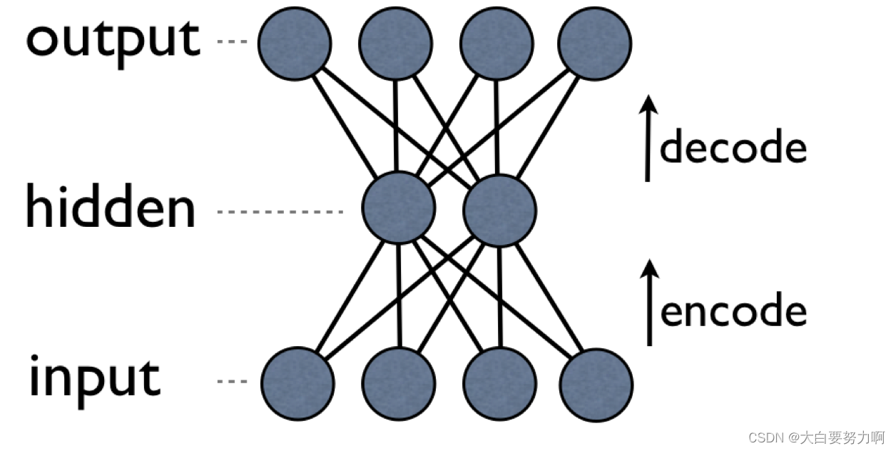
4.3 AutoEncoders

4.3.1 Auto encoders

Use the same example as input and output, i.e., they train a model for predicting an example from itself (using fewer variables)

Similar to PCA, but PCA provides only a linear transformation. ANNs can also create non-linear parameter transformations

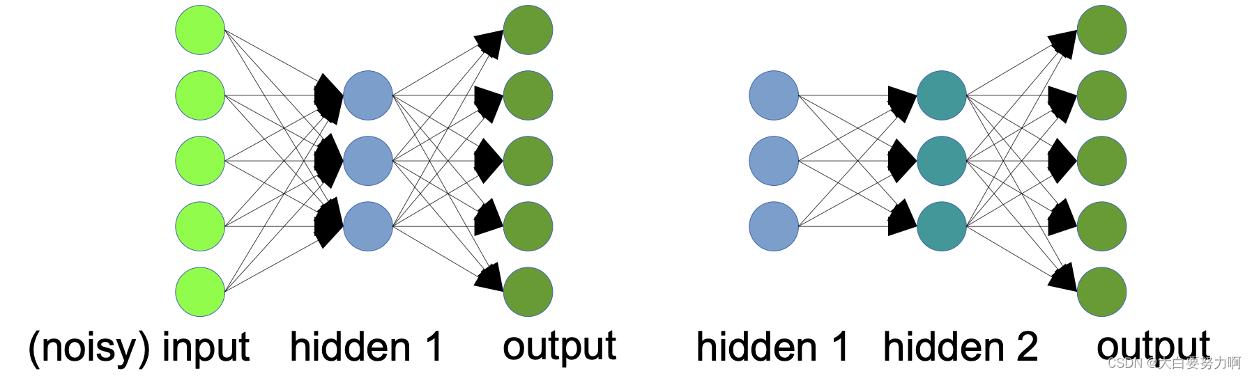
4.3.2 Denoising Auto Encoders

Instead of training with the same input and output, Denoising Auto Encoders add random noise to input and keep output clean
Result: A model that learns to remove noise from an instance

4.3.3 Stacked (Denoising) Auto Encoders

Stacked Auto Encoders contain several hidden layers
Hidden layers capture more complex hidden variables and/or denoising patterns. They are often trained consecutively:
First: train an auto encoder with one hidden layer
Second: train a second one-layer neural net (first hidden layer as input & original as output)

4.3.4 Auto Encoders for Outlier Detection

Also known as Replicator Neural Networks (Hawkins et al., 2002)
Train an autoencoder that captures the patterns in the data
Encode and decode each data point, measure deviation
Deviation is a measure for outlier score

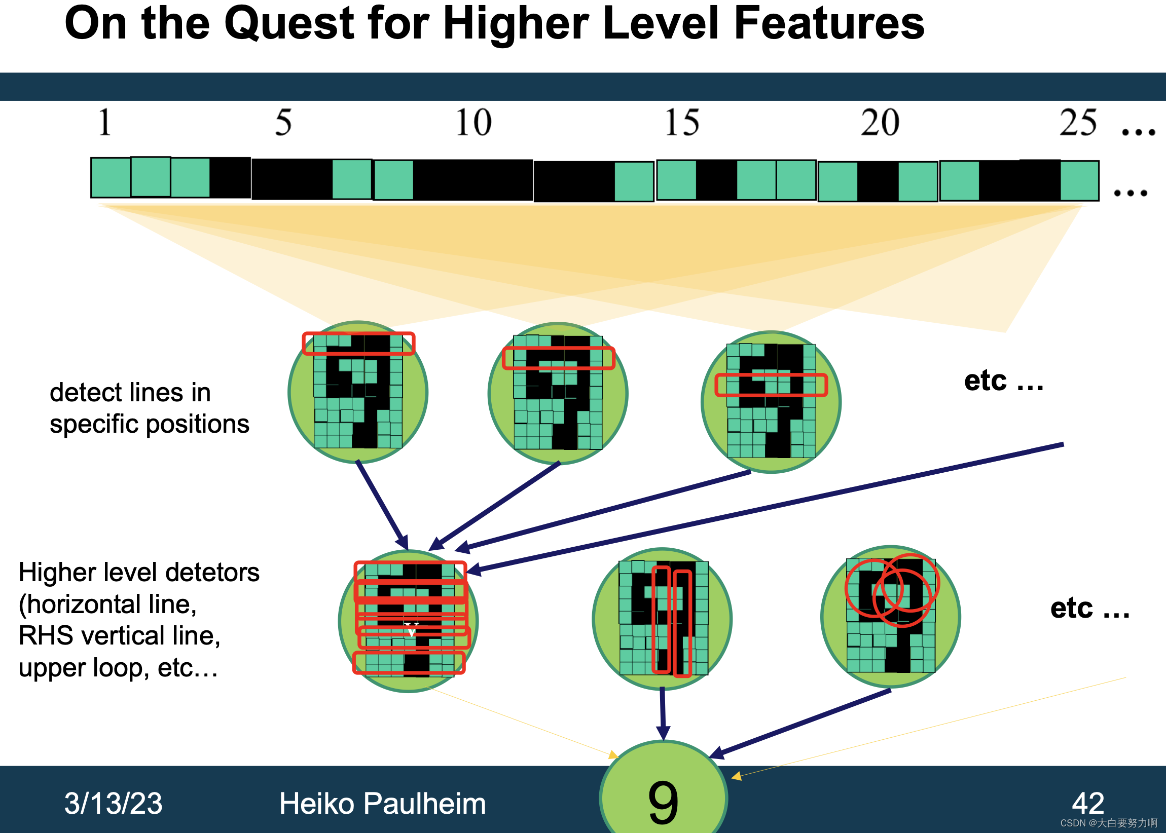
4.3.5 From Classifiers to Feature Detectors

What does a particular neuron in the hidden layer do?
Adjust weight -> strong signal for a horizontal line in the top row, ignoring everywhere else; strong signal for a dark area in the top left corner,… -> detect vertical lines / horizontal lines / circles …

Challenges: Positional variance, Color variance, …

4.4 Deep Learning

4.4.1 Memorizing vs. Learning

The goal of training a neural network is learning a generalized model should classify unseen examples

The opposite of generalization is memorization
Model learns training examples “by heart”
Lesser performance on unseen examples

Indicator: performance increase on training set, decrease on test set

Hidden layers define the capacity of a neural network
Roughly: how complex can the patterns be that are stored
more complex task -> more capacity need
Too low capacity: underfitting
Patterns that, e.g., separate classes have a certain complexity. We need enough hidden neuron connections to “store” those patterns

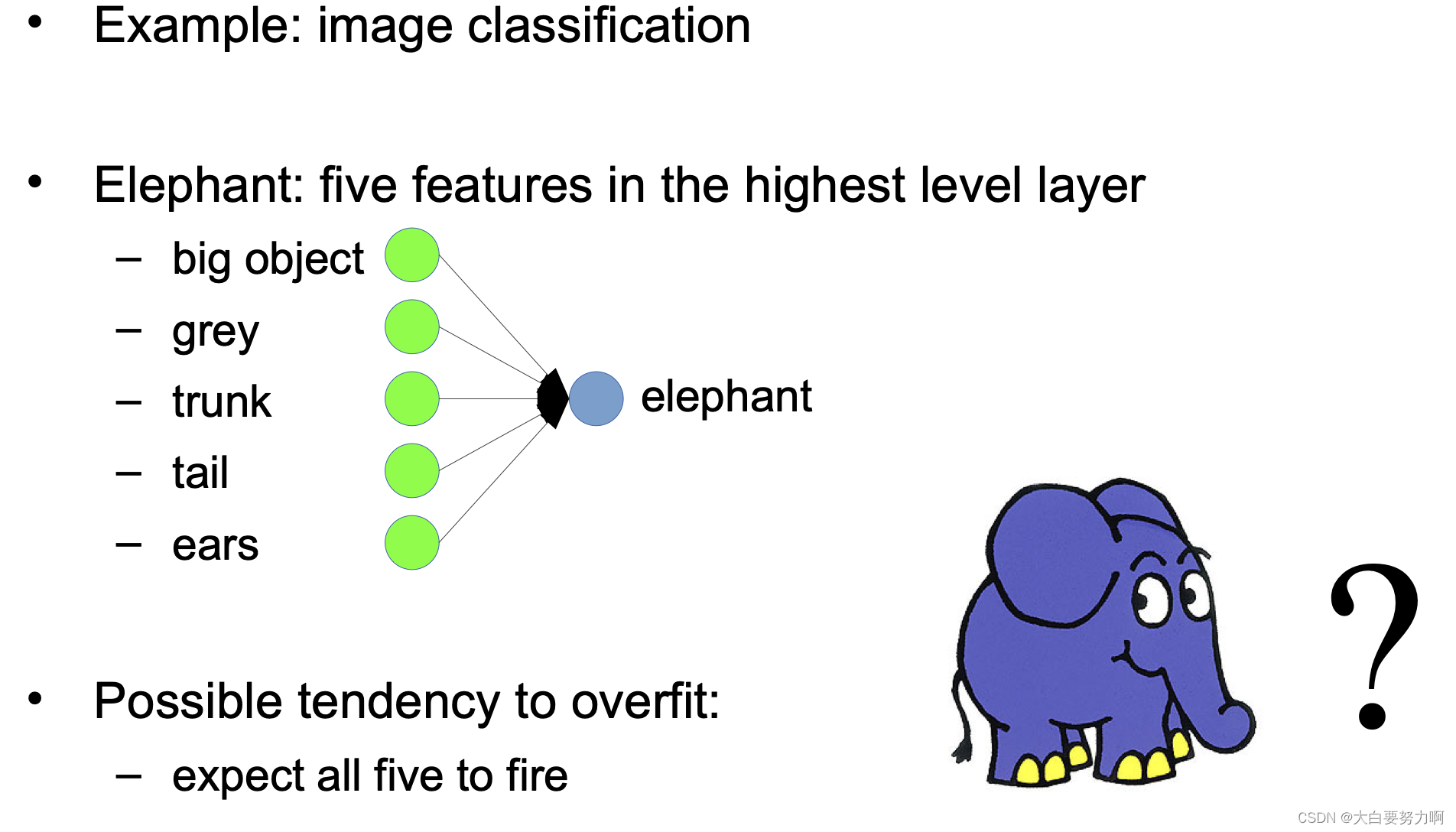
Too high capacity: overfitting
Examples can be identified by certain combinations of features. With enough hidden neuron connections, we can learn those combinations instead of generalized patterns

4.4.2 Regularization with Dropout

ANNs, and in particular Deep ANNs, tend to overfitting

Regularization
Randomly deactivate hidden neurons when training an example
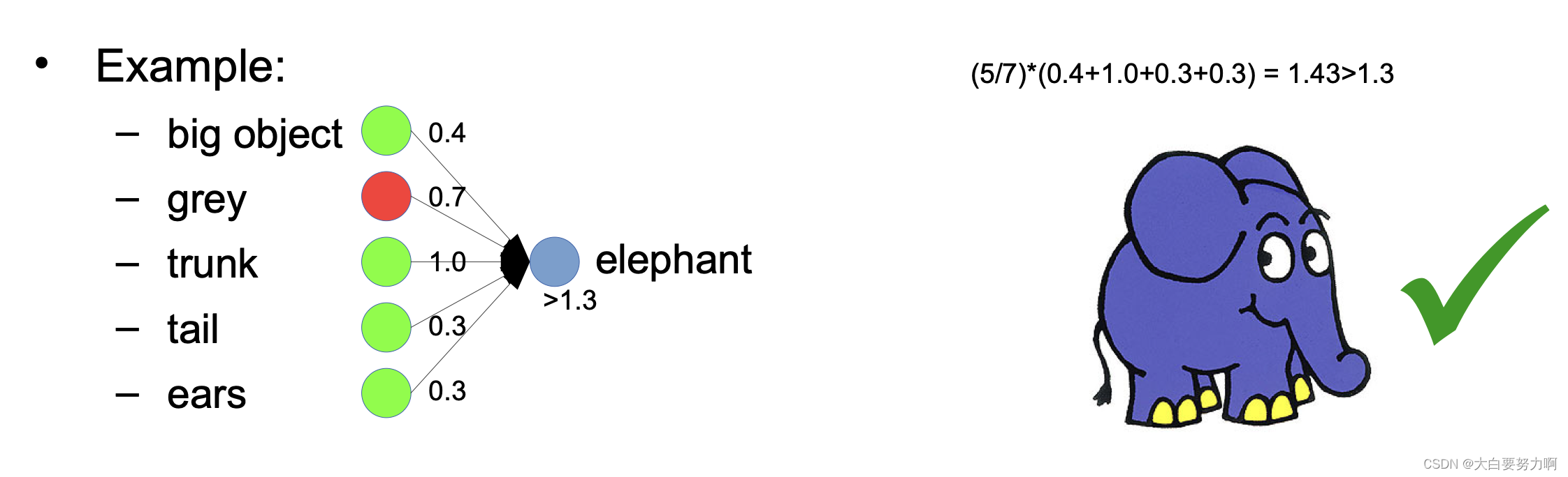
E.g., factor α=0.4: deactivate neurons randomly with probability 0.4

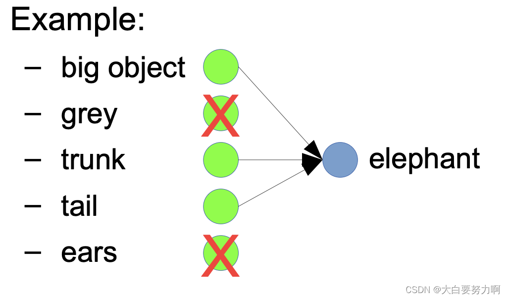
Result: Learned model is more robust, less overfit
For classification: use all hidden neurons
Problem: activation levels will be higher! –> Correction: multiply each output with 1/(1+α)

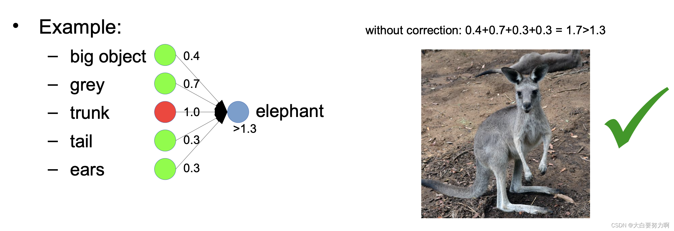
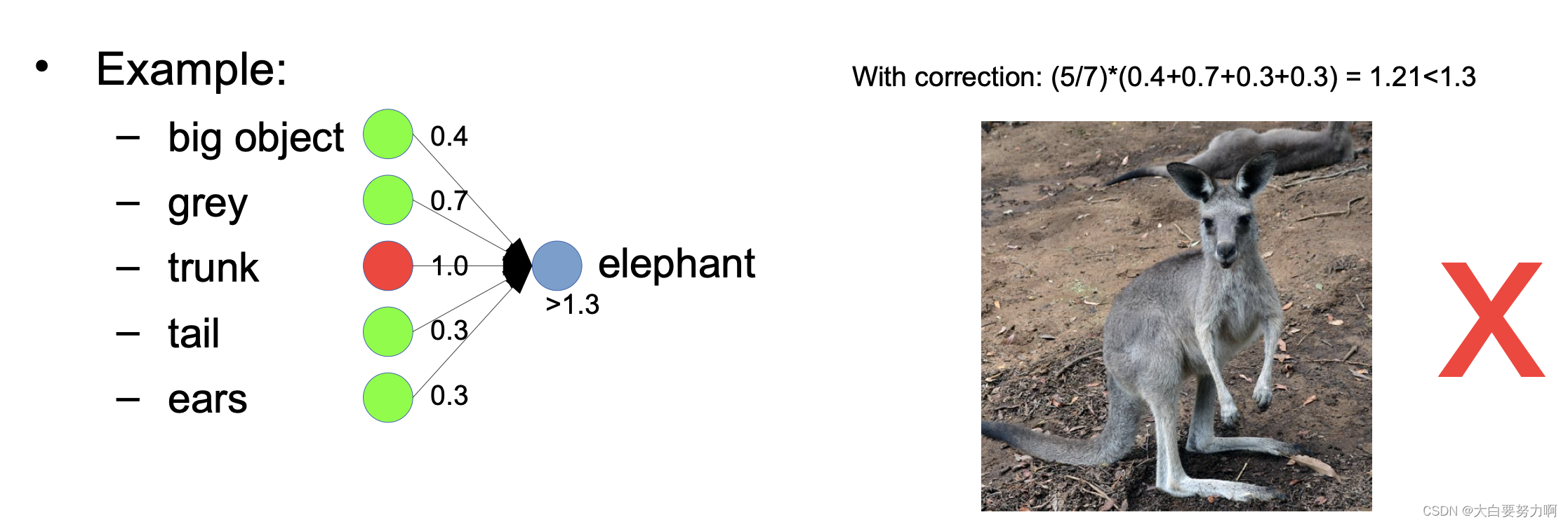
1/(1+α)=1/(1+0.4)=5/7

4.5 Network Architectures

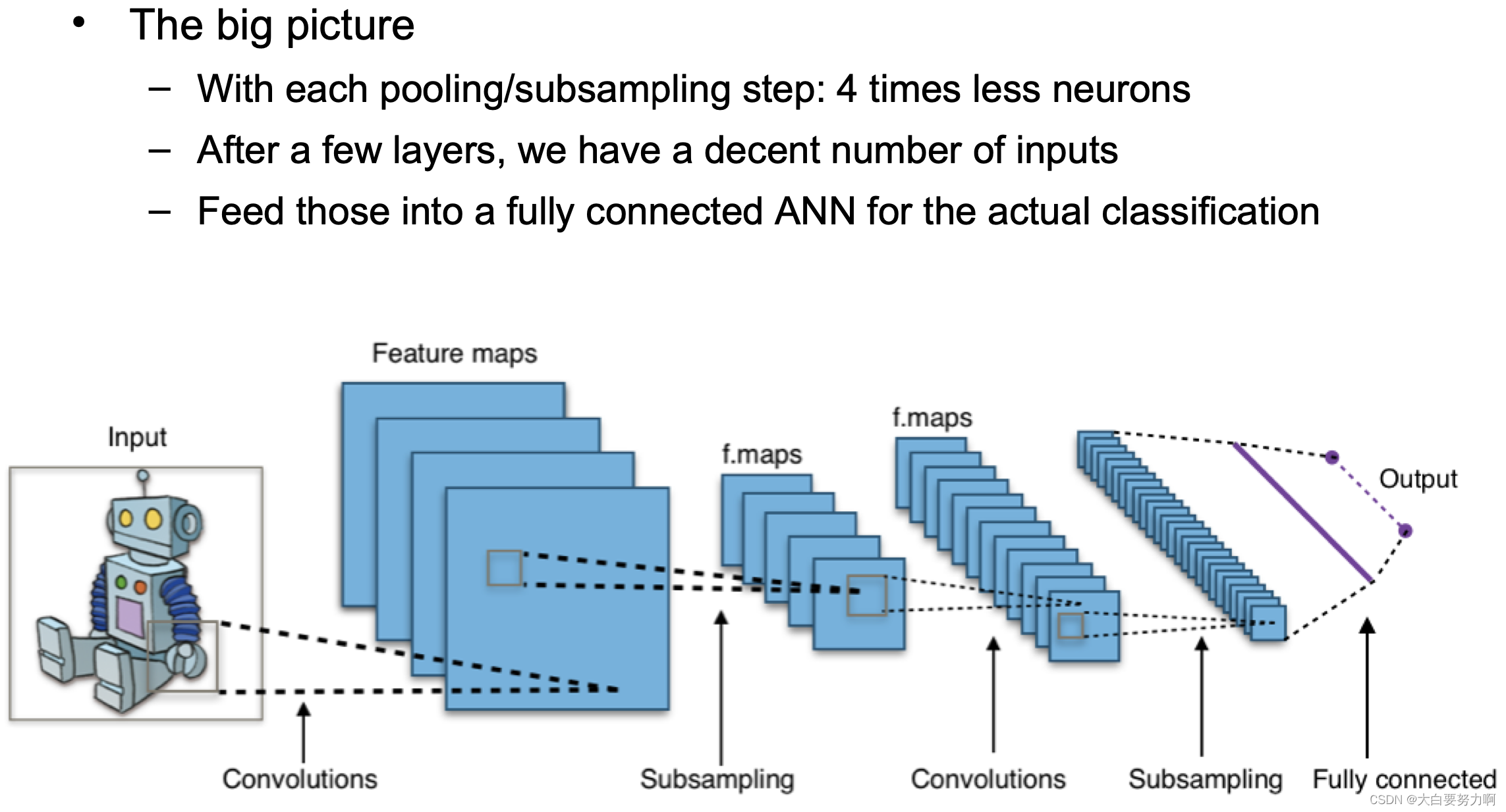
4.5.1 Architectures: Convolutional Neural Networks

Special architecture for image processing
Problem: imagine a 4k resolution picture (3840x2160)
Treating each pixel as an input: 8M input neurons and Connecting that to a hidden layer of the same size: 8M2 = 64 trillion weights to learn
This is hardly practical…

Solution: Convolutional neural networks

Two parts: Convolution layer + Pooling layer
Stacks of those are usually used

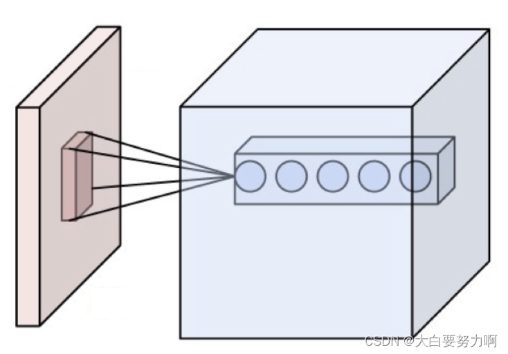
1. Convolution layer
Each neuron is connected to a small n x n square of the input neurons, i.e., number of connections is linear, not quadratic

Use different neurons for detecting different features
They can share their weights (intuition: a horizontal line looks the same everywhere)

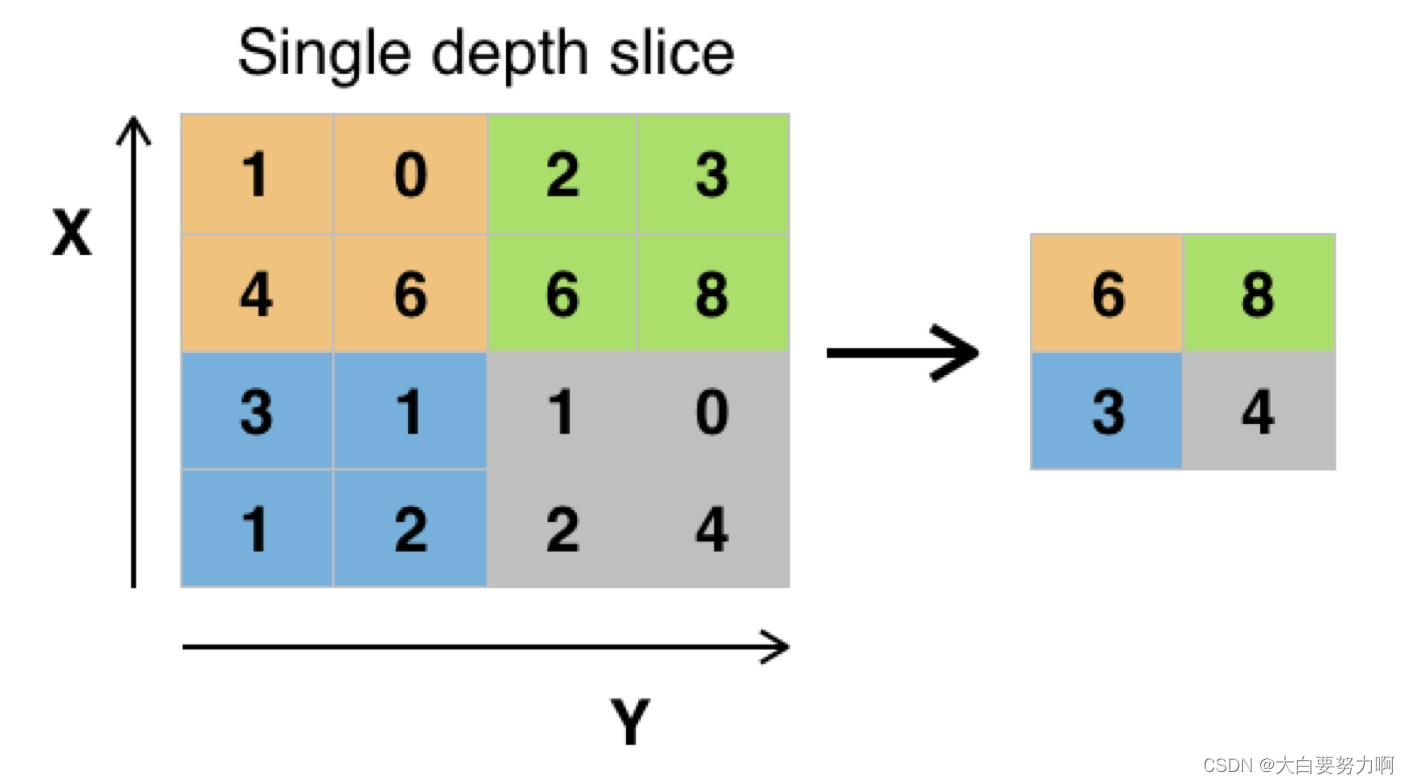
Pooling layer (aka subsampling layer)
Use only the maximum value of a neighborhood of neurons
Think:downsizing a picture
Number of neurons is divided by four with each pooling layer

The 4K picture revisited (3840x2160):
Treating each pixel as an input: 8M input neurons. Connecting that to a hidden layer of the same size: 8M^2 = 64 trillion weights to learn
Number of connections (weights to be learned) in the first convolutional layer: Assume each hidden neuron is connected to a 16x16 square and we learn 256 hidden features (i.e., 256 layers of convolutional neurons) 16x16x256x8M = still 526 billion weights
But: neurons for the same hidden feature share their weight. Thus, it’s just 16x16x256 = 65k weights

In practice, several layers are used.
Google’sGoogLeNet(Inception) - Current state of the art in image classification
Can be used as a pre-trained network

4.5.2 Possible Implications

Face Detection, Autonomous Driving, …

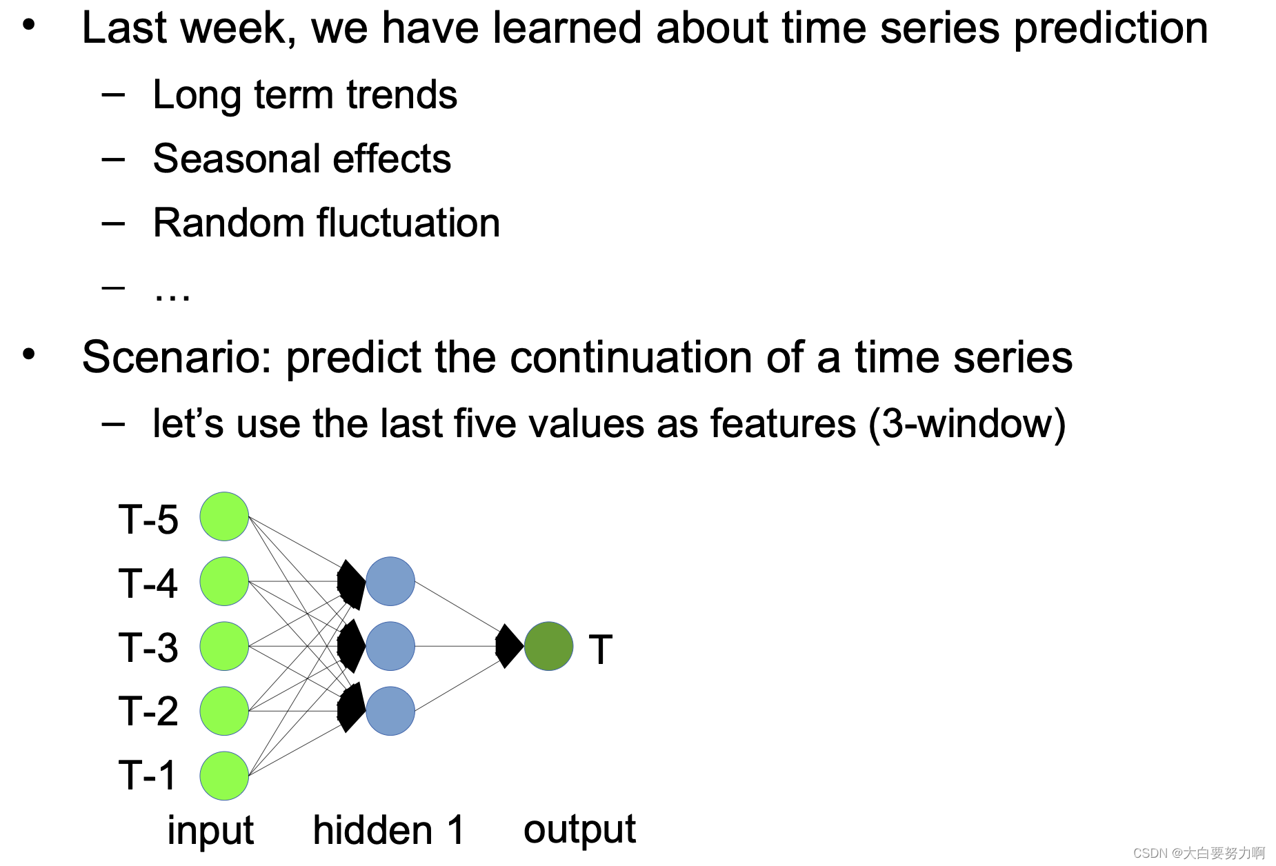
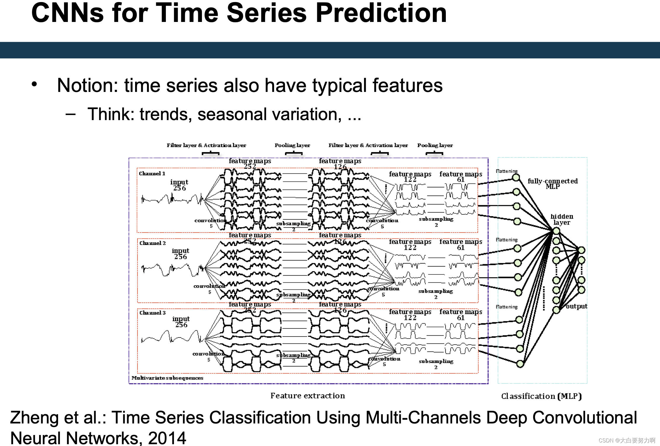
Using ANNs for Time Series Prediction

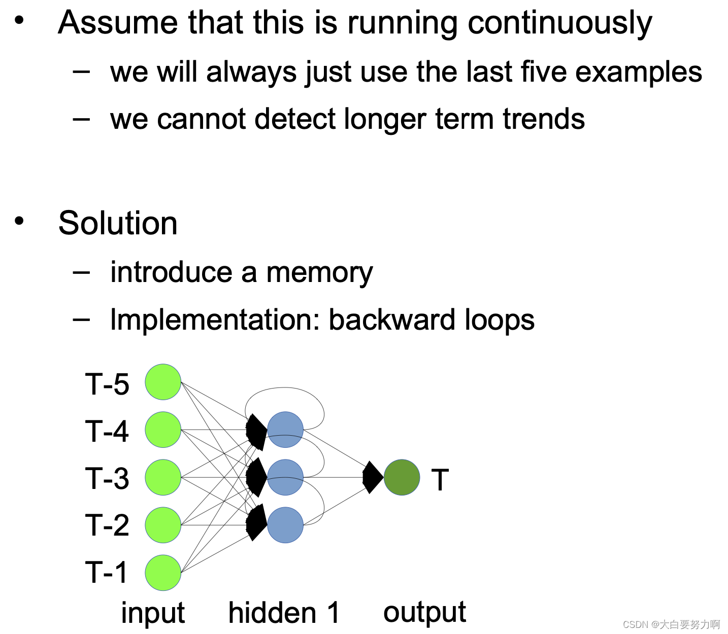
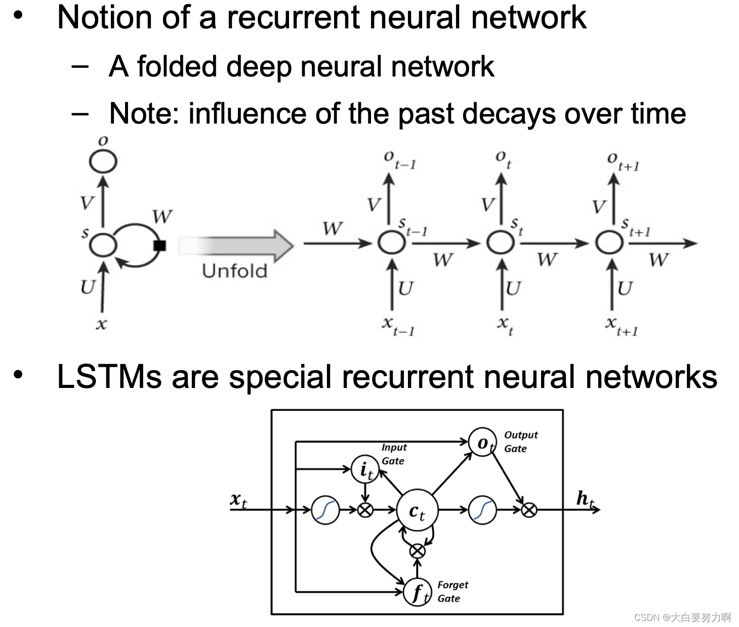
Long Short Term Memory Networks (LSTM)

Word2vec
word2vec is similar to an auto encoder for words
Training set: a text corpus
Training task variants:

• Continuous bag of words (CBOW): predict a word from the surrounding words
• Skip-Gram: predicts surrounding words of a word

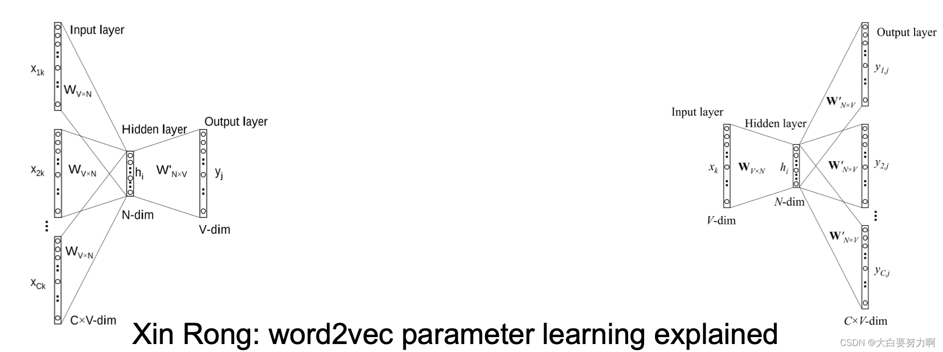
word2vec creates an n-dimensional vector for each word
Each word becomes a point in a vector space
Properties:
Similar words are positioned to each other
Relations have the same direction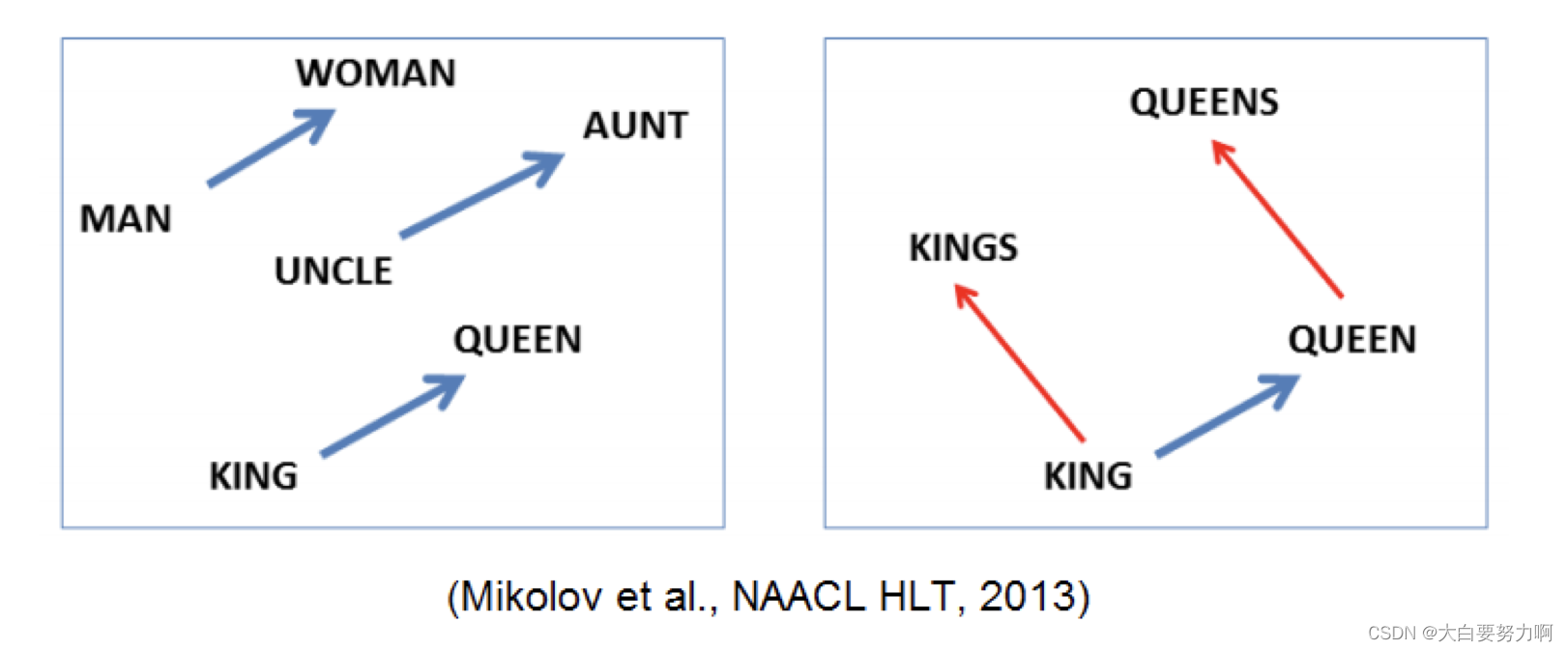

Arithmetics are possible in the vector space
king–man+woman≈queen
This allows for finding analogies:
king:man ↔ queen:woman
knee:leg ↔ elbow:forearm
Hillary Clinton:democrat ↔ Donald Trump:Republican

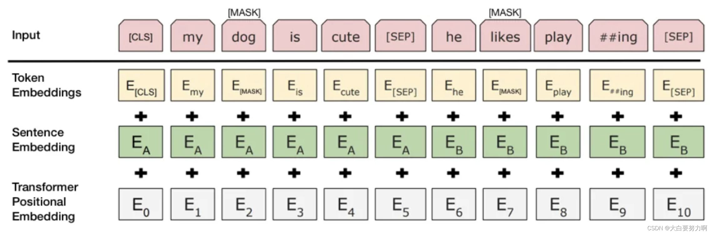
BERT
Learns a representation of words in context
Unlike word2vec: one fixed representation per word
Larger training corpus required

4.6 Transfer Learning with Neural Networks

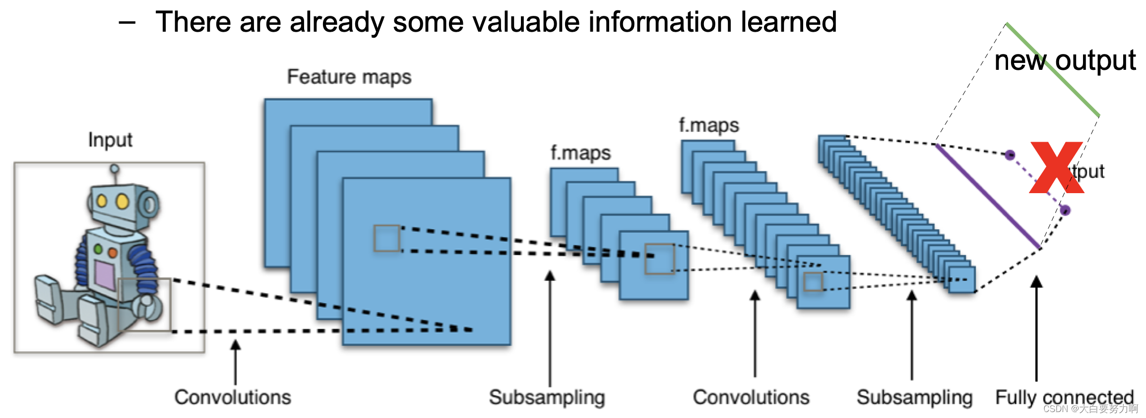
Reusing Pre-trained Networks
The output of a network can be used as an input to yet another classifier (neural network or other)
Think: a multi-label image classifier as an auto-encoder
Example: predict movie genre from poster
Using an image classifier trained for object recognition

In many cases, the last or second-to last layer are reused
Fine-tuning on a task at hand often leads to advantages, i.e., use the trained network, add a new classification layer, and present examples -> Referred to as “transfer learning”

Pre-trained neural networks can be (re)used for other tasks
They can also be retrained, using the pre-training as initialization Sometimes, different layers are frozen.
Rationale: There are already some valuable information learned

4.7 Summary