Pandas中Series数据的常用操作

1. 导包

In [1]: import numpy as np                                                                        
In [2]: import pandas as pd
In [3]: import matplotlib.pyplot as plt                                                                       

2. 创建对象

2.1 通过list方式创建（pandas默认自动生成整数索引）

In [4]: s1 = pd.Series([4,3,1,5,np.nan,'a',55])                                                  
In [5]: s1                                                                                       
Out[5]: 
0      4
1      3
2      1
3      5
4    NaN
5      a
6     55
dtype: object

In [6]: s2 = pd.Series(range(5,10))
In [7]: s2                                                                                       
Out[7]: 
0    5
1    6
2    7
3    8
4    9
dtype: int64

In [63]: np.random.seed(1)                                                                        
In [64]: s2 = pd.Series(np.random.randint(0, 7, size=10))                                          
In [65]: s2                                                                                        
Out[65]: 
0    5
1    3
2    4
3    0
4    1
5    3
6    5
7    0
8    0
9    1
dtype: int64

3. Series数据操作

3.1 统计

In [66]: s2.value_counts()        # 可用于绘制直方图                                                                 
Out[66]: 
0    3
5    2
3    2
1    2
4    1
dtype: int64

3.2 Series中str属性（封装了一系列的字符串操作方法）

In [67]: s = pd.Series(['A', 'B', 'C', 'Aaba', 'Baca', np.nan, 'CABA', 'dog', 'cat'])             

In [68]: s                                                                                        
Out[68]: 
0       A
1       B
2       C
3    Aaba
4    Baca
5     NaN
6    CABA
7     dog
8     cat
dtype: object

In [69]: s.str.lower()                                                                            
Out[69]: 
0       a
1       b
2       c
3    aaba
4    baca
5     NaN
6    caba
7     dog
8     cat
dtype: object

4. 时间序列(索引)

• pandas具有简单、强大和高效的时间处理函数，用于在频率转换时执行重采样操作。

In [151]: rng = pd.date_range('1/1/2019', periods=5, freq='D')   
In [152]: rng                      # 年月日时分秒：'Y'、'M'、'D'、'H'、'Min'、'S'                                                                                    
Out[152]: 
DatetimeIndex(['2019-01-01', '2019-01-02', '2019-01-03', '2019-01-04', '2019-01-05'],
              dtype='datetime64[ns]',
              freq='D')
In [153]: ts = pd.Series(np.random.randint(0, 500, len(rng)),index=rng)                           
In [154]: ts                                                                                      
Out[154]: 
2019-01-01    184
2019-01-02    443
2019-01-03    399
2019-01-04     24
2019-01-05    137
Freq: D, dtype: int64

In [162]: ts1 = ts.resample('9H').sum()      # 频率（9H）转换，执行 重采样 操作                                                     
In [163]: ts1                                                                                      
Out[163]: 
2019-01-01 00:00:00    184
2019-01-01 09:00:00      0
2019-01-01 18:00:00    443
2019-01-02 03:00:00      0
2019-01-02 12:00:00      0
2019-01-02 21:00:00    399
2019-01-03 06:00:00      0
2019-01-03 15:00:00     24
2019-01-04 00:00:00      0
2019-01-04 09:00:00      0
2019-01-04 18:00:00    137
Freq: 9H, dtype: int64

In [157]: tz = ts.tz_localize('UTC')         # 时区表示                                                       

In [158]: tz.tz_convert('US/Eastern')        # 转换成其它时区                                                      
Out[158]: 
2018-12-31 19:00:00-05:00    184
2019-01-01 19:00:00-05:00    443
2019-01-02 19:00:00-05:00    399
2019-01-03 19:00:00-05:00     24
2019-01-04 19:00:00-05:00    137
Freq: D, dtype: int64

In [178]: ts                    # 时间跨度转换                                                                  
Out[178]: 
2019-01-01    450
2019-01-02    199
2019-01-03    309
2019-01-04    325
2019-01-05    420
Freq: D, dtype: int64

In [179]: ps = ts.to_period()                                                                     

In [180]: ps                                                                                      
Out[180]: 
2019-01-01    450
2019-01-02    199
2019-01-03    309
2019-01-04    325
2019-01-05    420
Freq: D, dtype: int64

In [181]: ps.to_timestamp()                                                                       
Out[181]: 
2019-01-01    450
2019-01-02    199
2019-01-03    309
2019-01-04    325
2019-01-05    420
Freq: D, dtype: int64

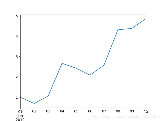
In [196]: ts = pd.Series(np.random.randn(10), index=pd.date_range('6/1/2019', periods=10))        

In [197]: ts                                                                                      
Out[197]: 
2019-06-01    0.999051
2019-06-02   -0.308171
2019-06-03    0.365838
2019-06-04    1.607507
2019-06-05   -0.238177
2019-06-06   -0.340828
2019-06-07    0.487594
2019-06-08    1.739073
2019-06-09    0.068970
2019-06-10    0.473241
Freq: D, dtype: float64

In [198]: ts = ts.cumsum()                                                                        

In [199]: ts                                                                                      
Out[199]: 
2019-06-01    0.999051
2019-06-02    0.690880
2019-06-03    1.056719
2019-06-04    2.664226
2019-06-05    2.426049
2019-06-06    2.085220
2019-06-07    2.572814
2019-06-08    4.311887
2019-06-09    4.380857
2019-06-10    4.854099
Freq: D, dtype: float64

In [200]: ts.plot()                                                                               
Out[200]: <matplotlib.axes._subplots.AxesSubplot at 0x7f04999e07b8>

In [201]: plt.show()       # 绘图如下：