


INF442 Amphi 5: Density estimation|Inheritance
依旧是无监督学习
1. Density Estimation
- 输入:n个点, P n = { p 1 , . . . , p n } ⊂ R d P_n=\{p_1,...,p_n\}\subset \mathbb{R}^d Pn={p1,...,pn}⊂Rd
- 我们假设这些点遵循一些分布: p i ∼ i i d ν p_i\sim_{iid} \nu pi∼iidν, ν \nu ν的density为 f : R d → R f:\mathbb{R}^d \to \mathbb{R} f:Rd→R
- 目的:从 P n P_n Pn中构建一个estimator f ^ n : R d → R \hat{f}_n: \mathbb{R}^d \to \mathbb{R} f^n:Rd→R来估计这些点的density。
- 应用:
- 去除噪声
- clustering(DBSCAN,mean-shift)
1.1 Quality of a density estimator
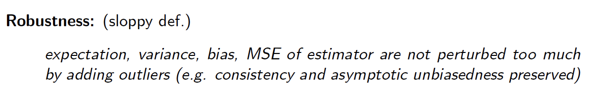
Bias, MSE, Convergence, Robustness
- 对于每一个固定的点 x ∈ R d x\in \mathbb{R}^d x∈Rd, f ^ n ( x ) \hat{f}_n(x) f^n(x)本身就是一个R中的随机变量(Random Variable)
- E P n ( f ^ n ( x ) ) \mathbb{E}_{P_n}(\hat{f}_n(x)) EPn(f^n(x))
- V a r P n ( f ^ n ( x ) ) \mathbb{Var}_{P_n}(\hat{f}_n(x)) VarPn(f^n(x))
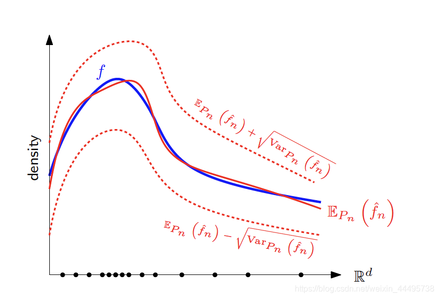
直觉:
-
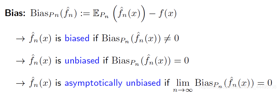
为了评价一个estimator,我们可以看它离目标的蓝线差多少 -> Bias
-
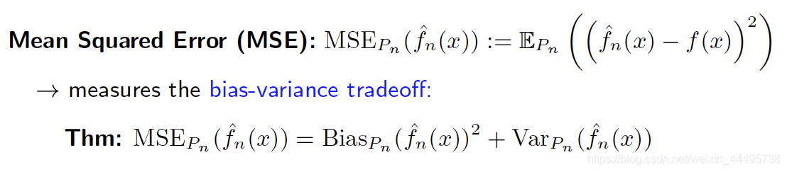
MSE (Mean Squared Error)
-
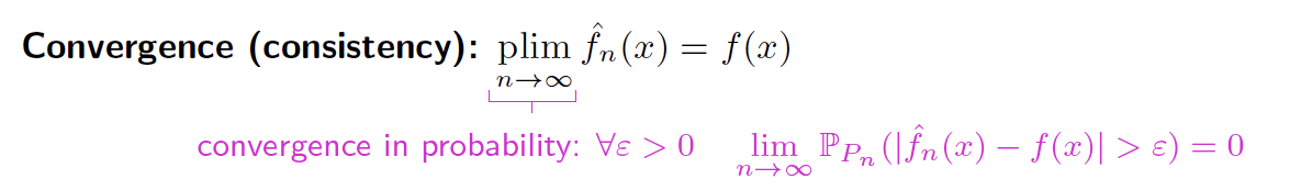
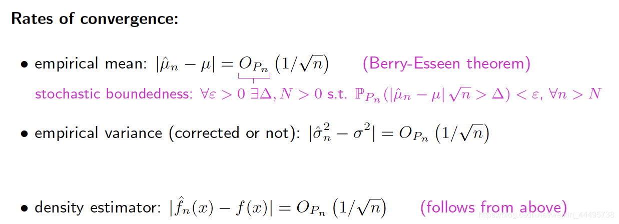
Convergence
性质:
如果MSE->0,则 f ^ n \hat{f}_n f^n是consistente的。(用Chebychev证明)。 -
Robusteness
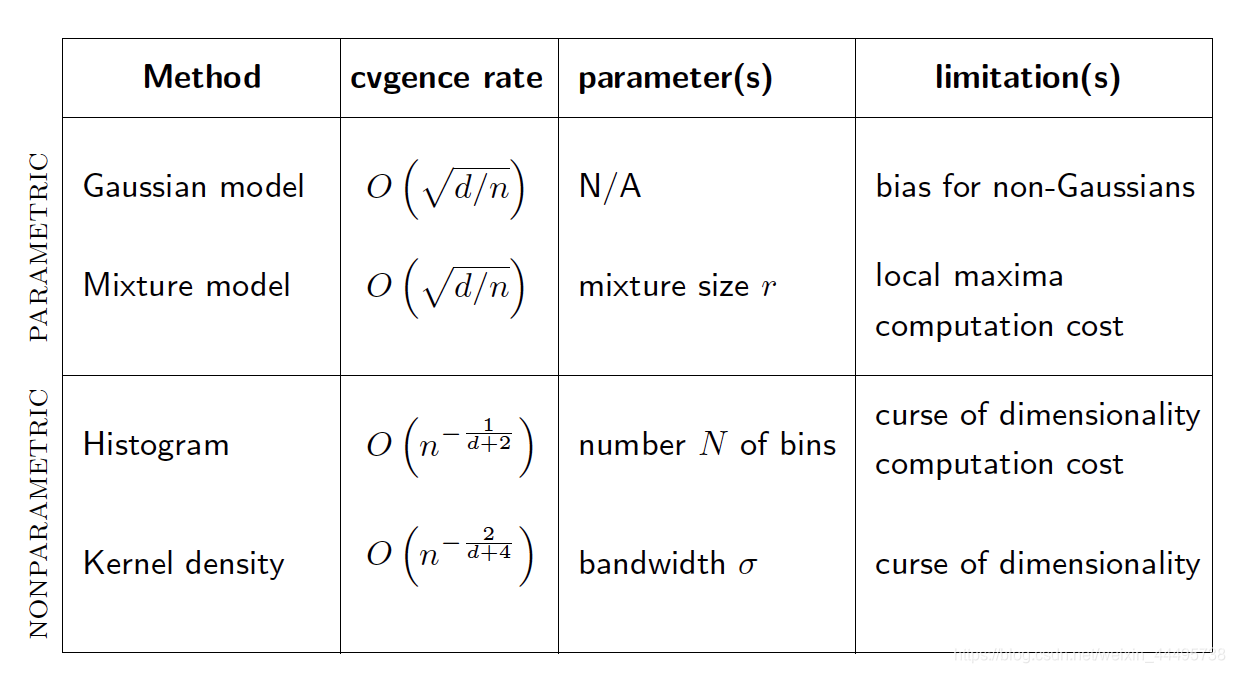
1.2 Parametric | Non-parametric Estimation
- Parametric estimator: 假设 ν \nu ν遵循某一个parametrized family,如Gaussian, Poisson, Exponential Families, etc.
- Nonparametric estimator: 点对点构建 f f f。如Histograms, Kernel Density Estimator, k-NN Estimator。
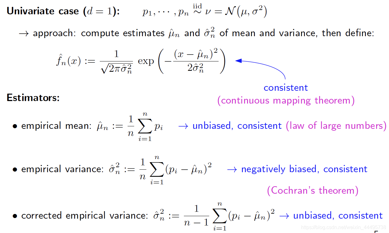
1.3 Parametric Method
1.3.1 Gaussian Model
单变量(d=1):
多变量:
d
>
1
d>1
d>1
- non-singular -> 可逆的
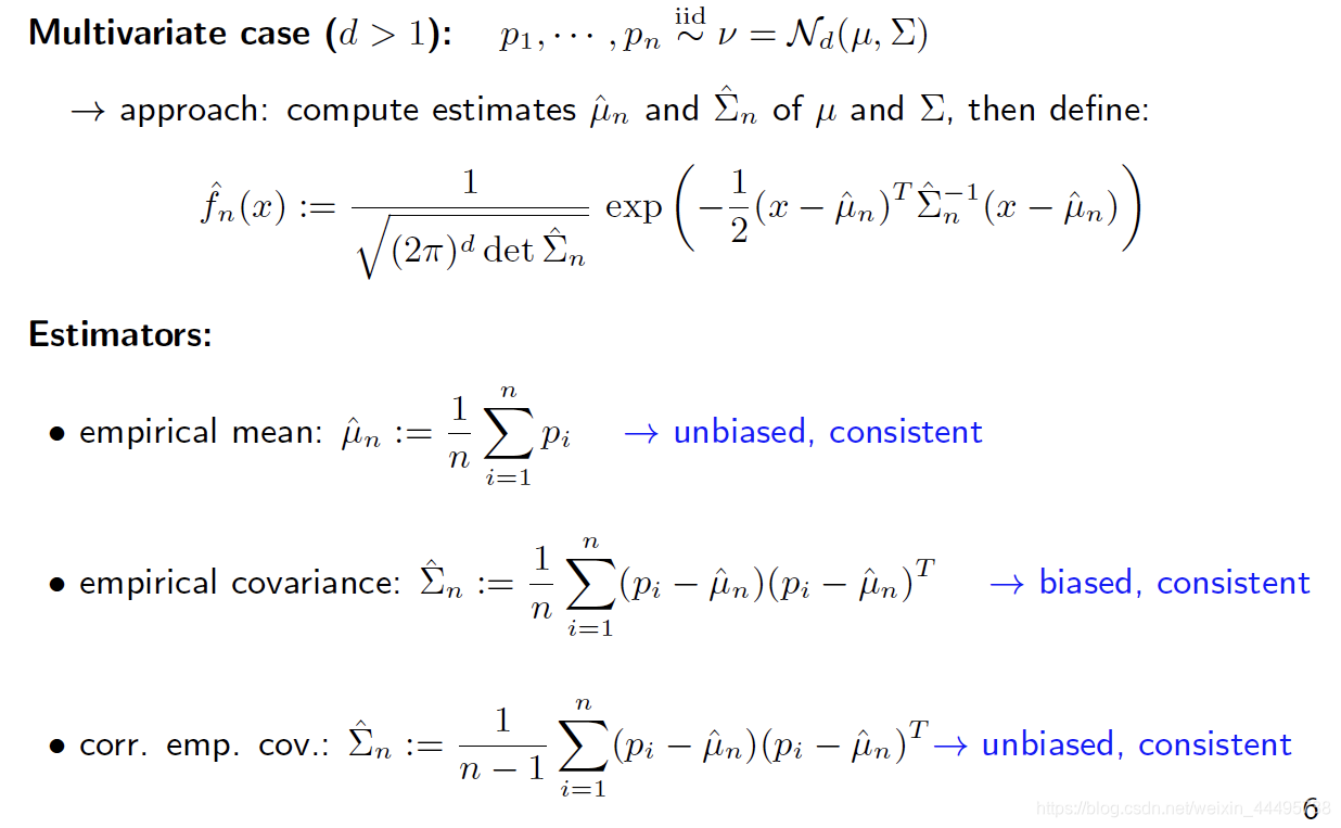
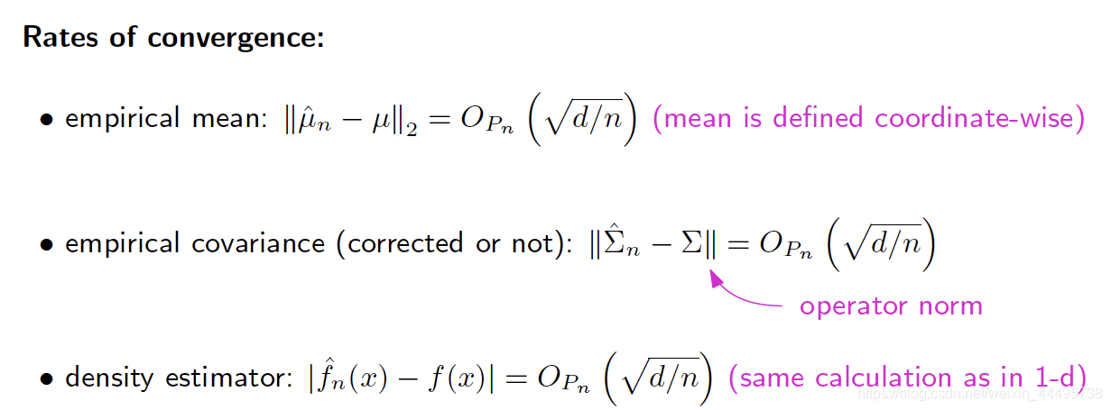
- dimension越大,收敛速度越慢
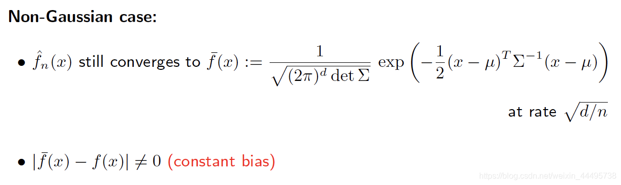
如果原始的Loi并不是Gaussien的:
1.3.2 Mixture Models
目的:去除因为原始的Loi不是Gaussien,单用Gaussien估计时产生的Bias。
方法:
用
r
r
r个density的加权方式得到
f ‾ ( x ) = ∑ i = 1 r ξ l ϕ l ( x ) \overline{f}(x)=\sum_{i=1}^r\xi_l \phi_l(x) f(x)=i=1∑rξlϕl(x)
- 每一个 ϕ l \phi_l ϕl都是一个probability density function (pdf)
- 每一个weight ξ ≥ 0 \xi\geq0 ξ≥0
- ∑ l = 1 r ξ l = 1 \sum_{l=1}^r \xi_l=1 ∑l=1rξl=1 [Combination Convex]
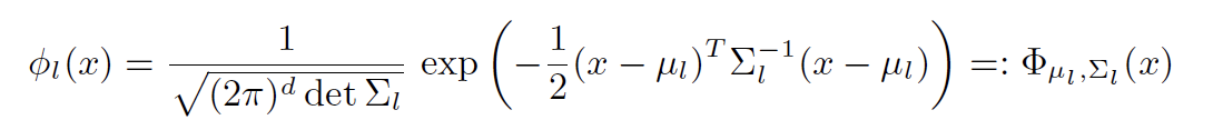
接下来我们研究GMM(Gaussian mix model):
- 即每一个
ϕ
l
\phi_l
ϕl的density都为
N
(
μ
l
,
∑
l
)
\mathcal{N}(\mu_l,\sum_l)
N(μl,∑l)
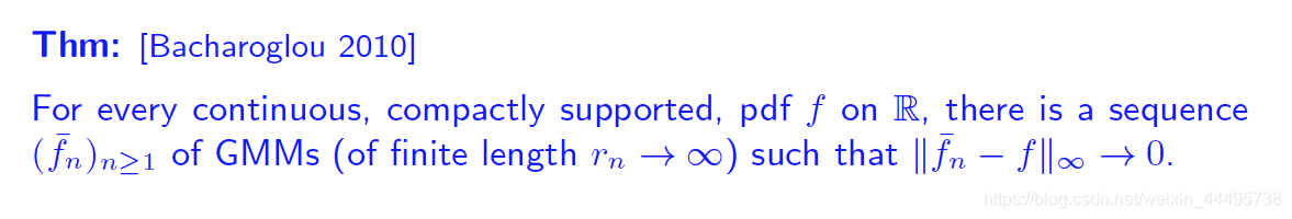
性质:
对于特定的f,总存在一个GMM的序列,其极限为 f f f。
[缺点是,这里下标n表示用n个Gaussian加权得到的 f n f_n fn]
想法: - 对于每一个固定的 r r r,我们尝试估计每一个组成成分的均值,方差,和其权重。
- 我们寻找在这些参数下使得这些点出现概率最大的参数。
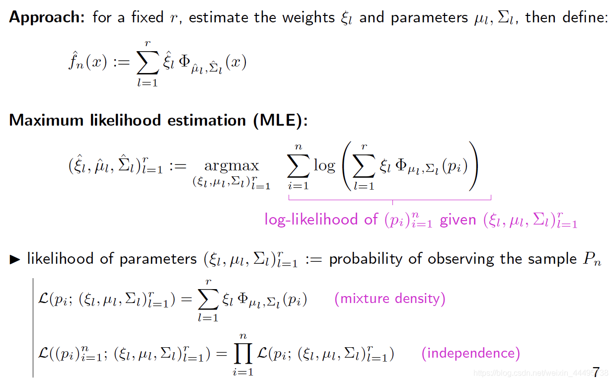
一些评价: - no closed-form solution
- non-concave functional -> local maxima, non-unique global maximum
- choice of mixture size r
- variational solvers (gradient ascent, Expectation-Maximization)
1.4 Non-parametric Method
1.4.1 Histograms
- tessellation:棋盘形布置
基本想法:
把 R d R^d Rd划分成若干个Grid,统计每一个Grid上observation出现的次数。
两种方法:
棋盘 / Voronoi Diagram
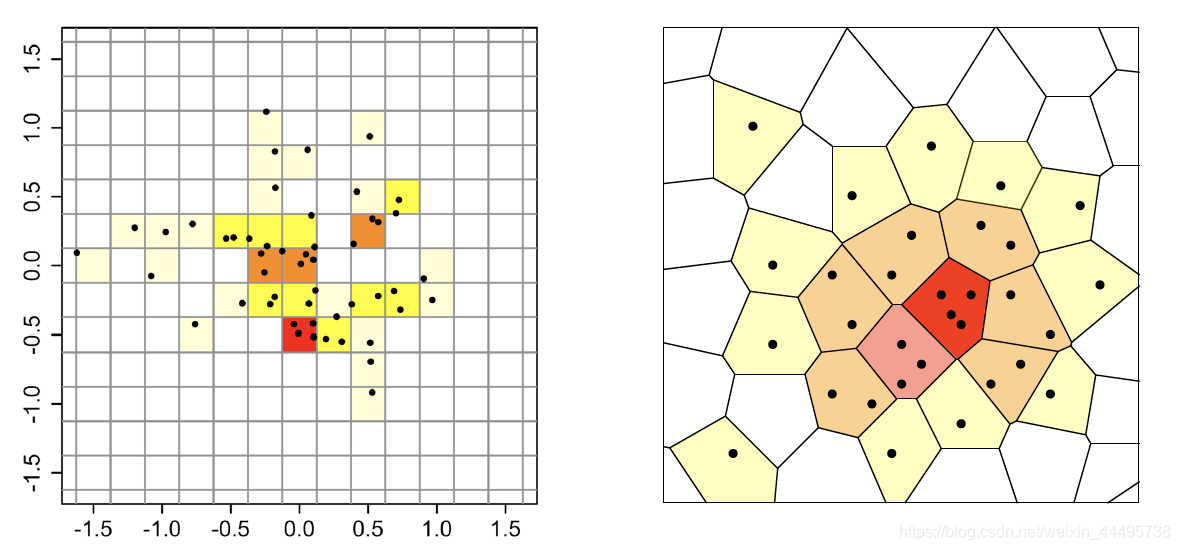
Uniform Grid
- 假设 P n ⊂ [ 0 , 1 ) d P_n \subset [0,1)^d Pn⊂[0,1)d,总共观察的数量为n。
- tessellate [ 0 , 1 ) d [0,1)^d [0,1)d with uniform grid of size N d N^d Nd,即整个空间是 1 1 1,一共有 N d N^d Nd个Cell,所以每一个Cell体积为 1 N d \frac{1}{N^d} Nd1。
- f ^ n ( x ) : = # observations in Cell(x) n V o l ( C e l l ( x ) ) = N d n ( ∑ i = 1 n 1 p i ∈ C e l l ( x ) ) \hat{f}_n(x):=\frac{\# \text{observations in Cell(x)}}{n Vol(Cell(x))}=\frac{N^d}{n}(\sum_{i=1}^n \mathbb{1}_{p_i\in Cell(x)}) f^n(x):=nVol(Cell(x))#observations in Cell(x)=nNd(∑i=1n1pi∈Cell(x)) (Vol是为了Voronoi中各个cell体积不一样的情况)
Bias
- 假设:f Lipschitiz-continue
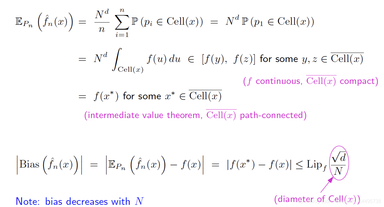
- 第二个等号是因为不同的点之间是iid的。
- 第三个等号源于f的定义,Borne的原因是因为f continue,Cell(x) compact
- 最后一个等号是积分的中值定理。
- 最后Bias的上界利用了f是Lipschitz这个条件。
∣ f ( x ∗ ) − f ( x ) ∣ ≤ L i p f ∣ x ∗ − x ∣ ≤ L i p f d N |f(x^*)-f(x)| \leq Lip_f |x^*-x| \leq Lip_f \frac{\sqrt{d}}{N} ∣f(x∗)−f(x)∣≤Lipf∣x∗−x∣≤LipfNd
- 当我们分的份数N越大,Bias越少。
推导过程解释:
因为每一个Cell的体积为
1
N
d
\frac{1}{N^d}
Nd1,其对角线长度为
(
1
N
+
1
N
+
⋯
+
1
N
)
1
d
=
d
N
(\frac{1}{N}+\frac{1}{N}+\dots+\frac{1}{N})^{\frac{1}{d}}=\frac{\sqrt{d}}{N}
(N1+N1+⋯+N1)d1=Nd。
- 为什么 x ∗ x^* x∗和 x x x在同一个Cell里面❓❓❓
Variance / MSE
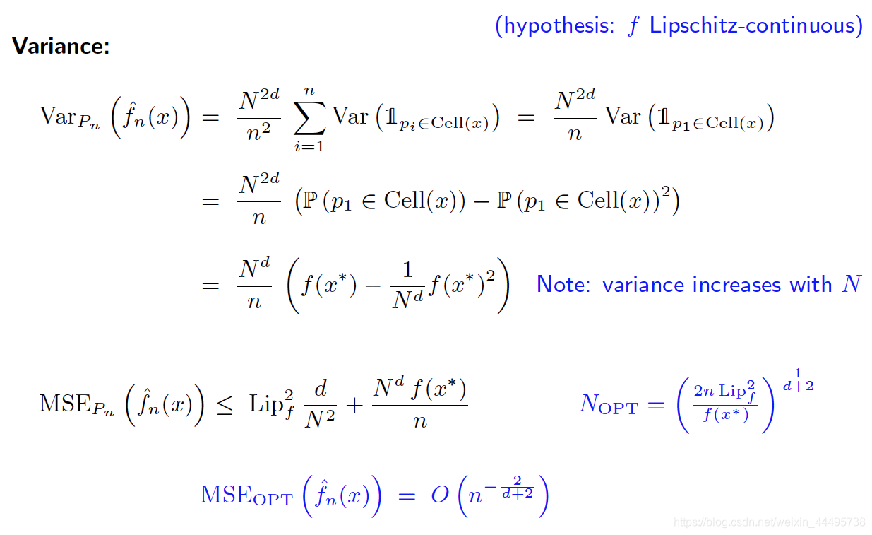
这里我们发现当我们N分的越大,Bias越少,但是Variance越大。-> Bias Variance Trade off。
取borne的下界,我们可以得到 N O P T N_{OPT} NOPT。
Rq:
- N O P T N_{OPT} NOPT一般在实践中是不知道的。
- Grid 并不适合 ν \nu ν的Support
1.4.2 Kernel Density Estimators
一般最常用的
对于每一个观察(黑线),加一个以其为中心的Gaussian。

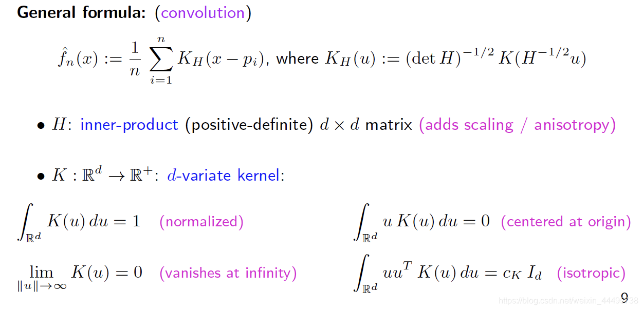
- Variate: 变量
研究一些特别的情况: -
H
=
σ
2
I
d
H = \sigma^2 I_d
H=σ2Id: Isotropic Kernel
- d e t ( H ) − 1 2 = σ − d I d det(H)^{-\frac{1}{2}}=\sigma^{-d}I_d det(H)−21=σ−dId
- H − 1 2 = σ − 1 I d H^{-\frac{1}{2}}=\sigma^{-1}I_d H−21=σ−1Id
- H − 1 2 u = H − 1 2 ( x − p i ) = x − p i σ H^{-\frac{1}{2}}u=H^{-\frac{1}{2}}(x-p_i)=\frac{x-p_i}{\sigma} H−21u=H−21(x−pi)=σx−pi
-
K
(
u
)
∝
k
(
∣
∣
u
∣
∣
2
2
)
,
k
:
R
+
→
R
+
K(u) \propto k(||u||_2^2),k:\mathbb{R}^+\to\mathbb{R}^+
K(u)∝k(∣∣u∣∣22),k:R+→R+
- normalizing factor c k , d = ( ∫ R d k ( ∣ ∣ u ∣ ∣ 2 2 ) d u ) − 1 c_{k,d}=(\int_{\mathbb{R}^d } k(||u||_2^2) du)^{-1} ck,d=(∫Rdk(∣∣u∣∣22)du)−1
因此,此时
f ^ n ( x ) : = 1 n ∑ i = 1 n k ( ∣ ∣ x − p i ∣ ∣ 2 2 σ 2 ) \hat{f}_n(x):=\frac{1}{n} \sum_{i=1}^n k(\frac{||x-p_i||_2^2}{\sigma^2}) f^n(x):=n1i=1∑nk(σ2∣∣x−pi∣∣22)
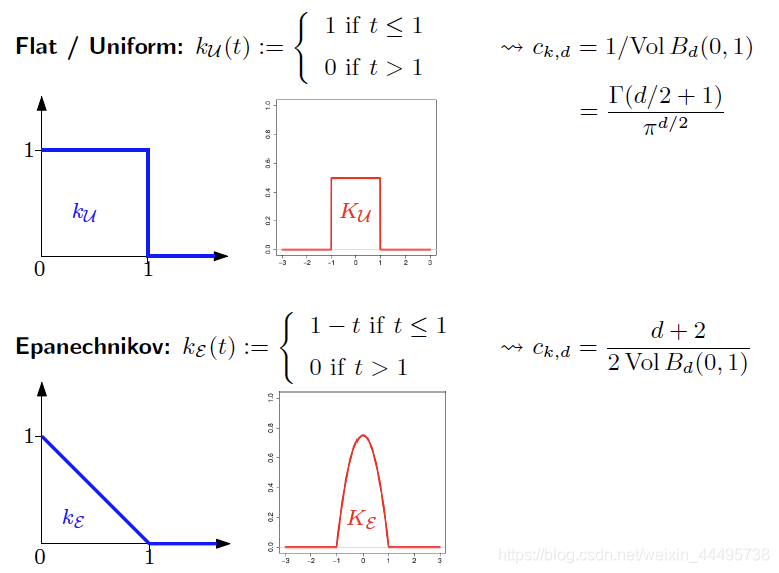
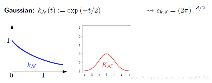
Common Kernels
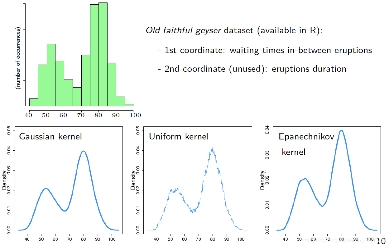
例子:间歇泉(geyser)
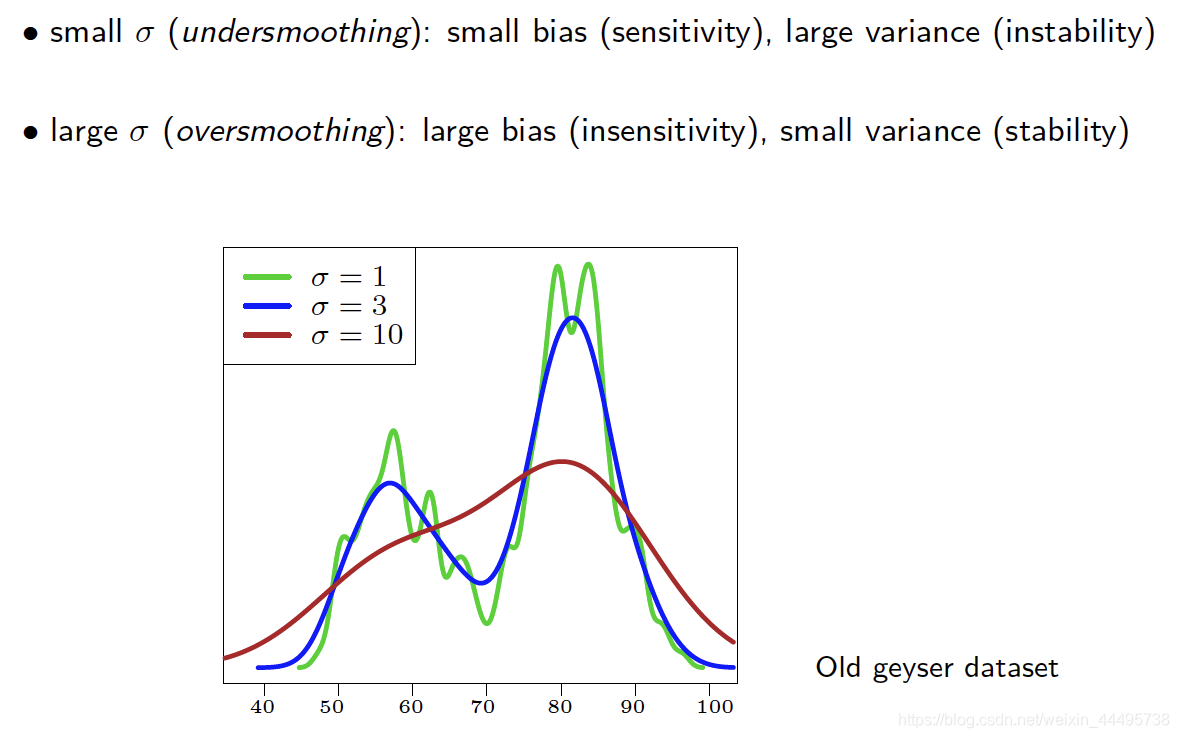
不同Bandwidth
σ
\sigma
σ下的影响
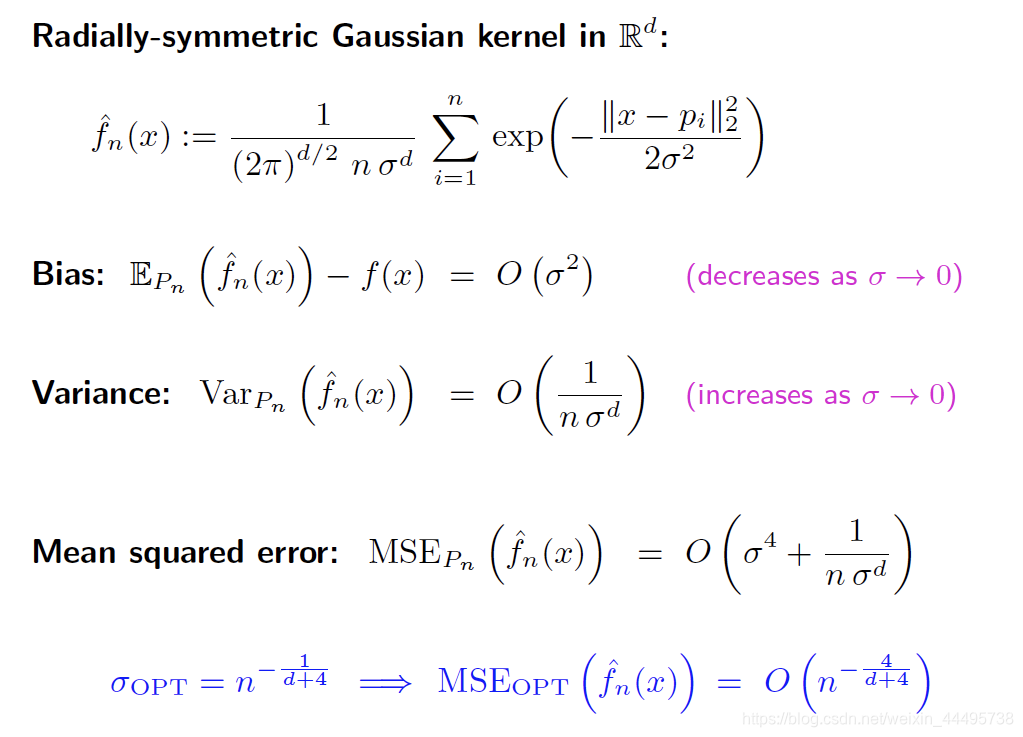
比之前的Histogramme收敛得更快:
之前的
M
S
E
=
O
(
n
−
2
d
+
2
)
MSE=O(n^{\frac{-2}{d+2}})
MSE=O(nd+2−2)
总结
2. Inheritance
2.1 基本的使用:
class B: public A,可以继承A的属性
class A{
	public:
	int i;
}
class B: public A{
	public:
	int j;
}

int main(){
	B b;
	b.i = 2;
	b.j = 4;
}
2.2 不同的Access Modifiers
左边的是父辈A中属性的类别,上面的是子辈继承父辈的方式:
class B : public Aclass B : protected A,则B中标记为public的方法也变为protected。class B : private A

例子:
class A {
public: int get_i () { return i; }
protected: int j;
private: int i;
};
class B : public A {
public: void print() {
std::cout << i; // error: i is private in A so hidden here
std::cout << j; // ok: j is protected in A so accessible here
std::cout << get_i(); // ok: get_i() is public in A so accessible here
}
};
int main () {
B b;
std::cout << b.i; // error: i is private in B
std::cout << b.j; // error: j is protected in B
std::cout << b.get_i(); // ok: get_i() is public in B
return 0;
}
2.3 Inheritance and constructors / destructors
- 构建的时候是从父辈的Constructor开始。
- 消除的时候是从子辈的Destructor开始。
class A {
public:
A () { std::cout << "ctor A" << std::endl; }
A () { std::cout << "dtor A" << std::endl; }
};
class B : public A {
public:
B () { std::cout << "ctor B" << std::endl; }
B () { std::cout << "dtor B" << std::endl; }
};
int main () {
B b; // prints "ctor A" then "ctor B"
return 0;
} // prints "dtor B" then "dtor A"
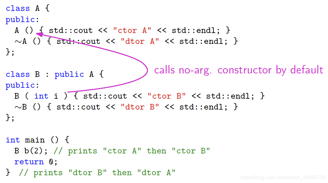
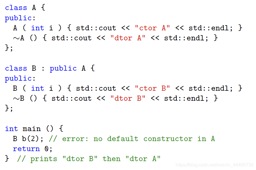
错误的原因是在B中运行constutor的时候调用的是其父辈A默认的constructor A()。但是这里只有A(int i) [A() 默认消失了]
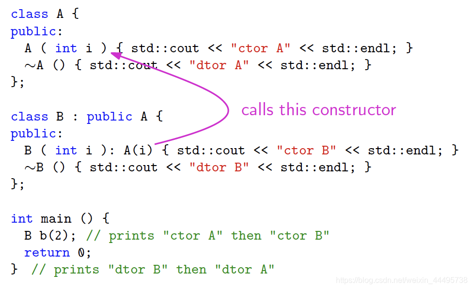
B(int i):A(i):将B的constructor和A的某一个特定的constructor相联系在一起。
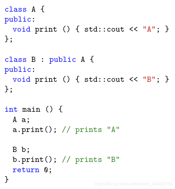
2.4 Virtual Functions
这里B继承了A,但是B中也有一个和A中一样的函数print。此时b.print()执行的是B中的print函数。
普通函数
Virtual Function
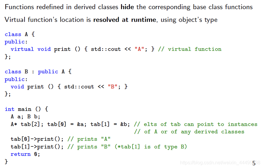
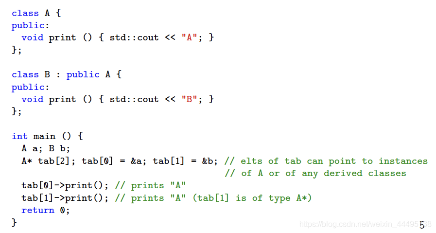
我们可以定义一个数组,
A* tab[3]; tab[0]=&a; tab[1]=&b; tab[2]=&c;,即他的子辈都可以转换到父辈的类型,从而构建一个数组。
普通Functions’s location is resolved at compile time ,即用的是变量的类型。
Virtual Frunction’s location is resolved at runtime,用的是object的类型。
Virtual Function使用缺点:
- 比较耗时,当继承关系比较复杂的情况下。
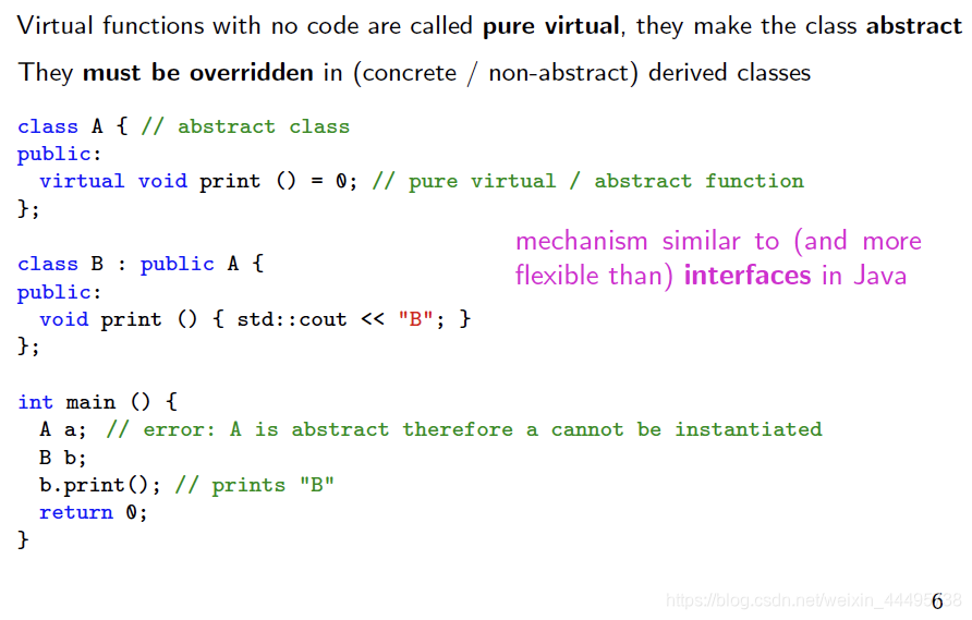
2.5 Pure virtual (abstract) functions
这个类似于Java中的Interace
- 一个只有pur virtual的父辈是abstract的。
- 它们不能被Instantiate,所有的抽象的方法要子辈implement。
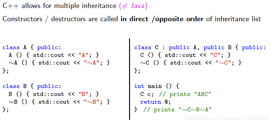
2.6 Multiple inheritance
C++中一个类别可以有多个父辈,但Java中不行
Deconstructor的顺序和Constructor的顺序正好相反。
因为C++中一个类别可以有多个父辈,所以会产生DIamond Problem,即如果不用Virtual Function,子辈中会有多个父辈。
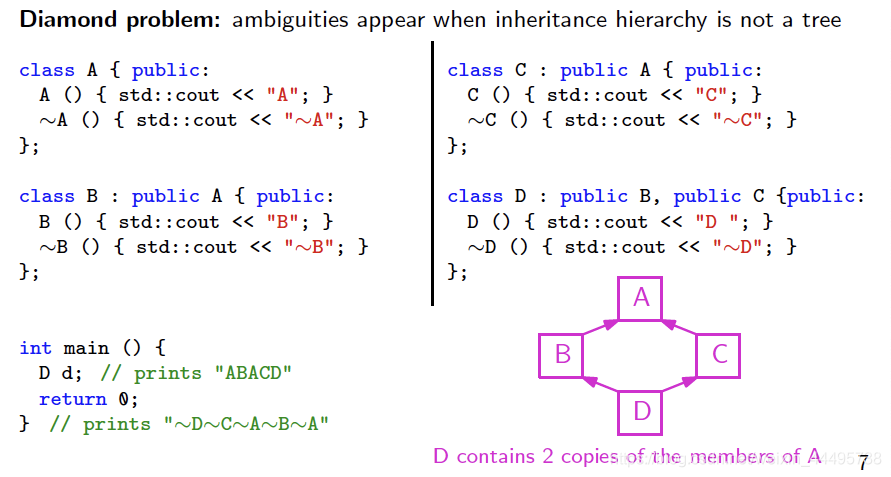
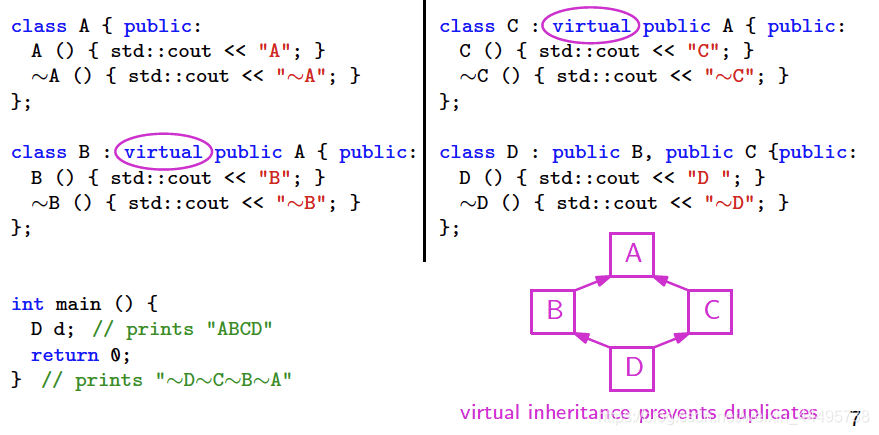
总结来说:
若A->B,A->C,即A有多个子辈,则A所有子辈在继承时都要加上virtual这个关键字。
class B: virtual public A


 338
338

 被折叠的 条评论
为什么被折叠?
被折叠的 条评论
为什么被折叠?
 到【灌水乐园】发言


