


数据分析-学术前沿趋势分析
任务1:论文数据统计
任务说明
任务主题:论文数量统计,即统计2019年全年计算机各个方向论文数量;
任务内容:赛题的理解、使用 Pandas 读取数据并进行统计;
任务成果:学习 Pandas 的基础操作;
具体代码实现
导入需要的python包
#导入包
import pandas as pd #数据处理,数据分析
import matplotlib.pyplot as plt #画图工具
import seaborn as sns #画图工具
from bs4 import BeautifulSoup #用于爬取arxiv的数据
import json #读取数据,数据为json格式
import re #用于正则表达式,匹配字符串的模式
读取数据
#读取数据
data= [] #列表用于存储读入的数据

#使用with语句优势:1.自动关闭文件句柄;2.自动显示(处理)文件读取数据异常
with open("arxiv-metadata-oai-snapshot.json", 'r') as f:
    for idx, line in enumerate(f):
        ## 读取前100行后,停止
        if idx >=100:
            break
        data.append(json.loads(line))#将数据加载到data列表中

data = pd.DataFrame(data)#将列表转换为dataframe格式,方便pandas分析。pandas两种格式series和dataframe
data.shape#显示数据大小
(100, 14)
数据预处理
首先我们先来粗略统计论文的种类信息:
count:一列数据的元素个数;
unique:一列数据中元素的种类;
top:一列数据中出现频率最高的元素;
freq:一列数据中出现频率最高的元素的个数;
data["categories"].describe()
count      1796911
unique       62055
top       astro-ph
freq         86914
Name: categories, dtype: object
判断共出现多少独立种类
# 所有的种类(独⽴的)
unique_categories = set([i for l in [x.split(' ') for x in data["categories"]]
for i in l])
len(unique_categories)
unique_categories
{'acc-phys',
 'adap-org',
 'alg-geom',
 'ao-sci',
 'astro-ph',
 'astro-ph.CO',
 'astro-ph.EP',
 'astro-ph.GA',
 'astro-ph.HE',
 'astro-ph.IM',
 'astro-ph.SR',
 'atom-ph',
 'bayes-an',
 'chao-dyn',
 'chem-ph',
 'cmp-lg',
 'comp-gas',
 'cond-mat',
 'cond-mat.dis-nn',
 'cond-mat.mes-hall',
 'cond-mat.mtrl-sci',
 'cond-mat.other',
 'cond-mat.quant-gas',
 'cond-mat.soft',
 'cond-mat.stat-mech',
 'cond-mat.str-el',
 'cond-mat.supr-con',
 'cs.AI',
 'cs.AR',
 'cs.CC',
 'cs.CE',
 'cs.CG',
 'cs.CL',
 'cs.CR',
 'cs.CV',
 'cs.CY',
 'cs.DB',
 'cs.DC',
 'cs.DL',
 'cs.DM',
 'cs.DS',
 'cs.ET',
 'cs.FL',
 'cs.GL',
 'cs.GR',
 'cs.GT',
 'cs.HC',
 'cs.IR',
 'cs.IT',
 'cs.LG',
 'cs.LO',
 'cs.MA',
 'cs.MM',
 'cs.MS',
 'cs.NA',
 'cs.NE',
 'cs.NI',
 'cs.OH',
 'cs.OS',
 'cs.PF',
 'cs.PL',
 'cs.RO',
 'cs.SC',
 'cs.SD',
 'cs.SE',
 'cs.SI',
 'cs.SY',
 'dg-ga',
 'econ.EM',
 'econ.GN',
 'econ.TH',
 'eess.AS',
 'eess.IV',
 'eess.SP',
 'eess.SY',
 'funct-an',
 'gr-qc',
 'hep-ex',
 'hep-lat',
 'hep-ph',
 'hep-th',
 'math-ph',
 'math.AC',
 'math.AG',
 'math.AP',
 'math.AT',
 'math.CA',
 'math.CO',
 'math.CT',
 'math.CV',
 'math.DG',
 'math.DS',
 'math.FA',
 'math.GM',
 'math.GN',
 'math.GR',
 'math.GT',
 'math.HO',
 'math.IT',
 'math.KT',
 'math.LO',
 'math.MG',
 'math.MP',
 'math.NA',
 'math.NT',
 'math.OA',
 'math.OC',
 'math.PR',
 'math.QA',
 'math.RA',
 'math.RT',
 'math.SG',
 'math.SP',
 'math.ST',
 'mtrl-th',
 'nlin.AO',
 'nlin.CD',
 'nlin.CG',
 'nlin.PS',
 'nlin.SI',
 'nucl-ex',
 'nucl-th',
 'patt-sol',
 'physics.acc-ph',
 'physics.ao-ph',
 'physics.app-ph',
 'physics.atm-clus',
 'physics.atom-ph',
 'physics.bio-ph',
 'physics.chem-ph',
 'physics.class-ph',
 'physics.comp-ph',
 'physics.data-an',
 'physics.ed-ph',
 'physics.flu-dyn',
 'physics.gen-ph',
 'physics.geo-ph',
 'physics.hist-ph',
 'physics.ins-det',
 'physics.med-ph',
 'physics.optics',
 'physics.plasm-ph',
 'physics.pop-ph',
 'physics.soc-ph',
 'physics.space-ph',
 'plasm-ph',
 'q-alg',
 'q-bio',
 'q-bio.BM',
 'q-bio.CB',
 'q-bio.GN',
 'q-bio.MN',
 'q-bio.NC',
 'q-bio.OT',
 'q-bio.PE',
 'q-bio.QM',
 'q-bio.SC',
 'q-bio.TO',
 'q-fin.CP',
 'q-fin.EC',
 'q-fin.GN',
 'q-fin.MF',
 'q-fin.PM',
 'q-fin.PR',
 'q-fin.RM',
 'q-fin.ST',
 'q-fin.TR',
 'quant-ph',
 'solv-int',
 'stat.AP',
 'stat.CO',
 'stat.ME',
 'stat.ML',
 'stat.OT',
 'stat.TH',
 'supr-con'}
我们的任务要求对于2019年以后的paper进行分析,所以首先对于时间特征进行预处理,从而得到2019年以后的所有种类的论文:
data["year"] = pd.to_datetime(data["update_date"]).dt.year #将update_date从例如2019-02-20的str变为datetime格式,并提取处year
del data["update_date"] #删除 update_date特征,其使命已完成
data = data[data["year"] >= 2019] #找出 year 中2019年以后的数据,并将其他数据删除

# data.groupby(['categories','year']) #以 categories 进行排序,如果同一个categories 相同则使用 year 特征进行排序
data.reset_index(drop=True, inplace=True) #重新编号
data #查看结果
 	id 	categories 	year
0 	0704.0297 	astro-ph 	2019
1 	0704.0342 	math.AT 	2019
2 	0704.0360 	astro-ph 	2019
3 	0704.0525 	gr-qc 	2019
4 	0704.0535 	astro-ph 	2019
... 	... 	... 	...
395118 	quant-ph/9911051 	quant-ph 	2020
395119 	solv-int/9511005 	solv-int nlin.SI 	2019
395120 	solv-int/9809008 	solv-int nlin.SI 	2019
395121 	solv-int/9909010 	solv-int adap-org hep-th nlin.AO nlin.SI 	2019
395122 	solv-int/9909014 	solv-int nlin.SI 	2019
下面我们挑选出计算机领域内的所有文章:
#爬取所有的类别
website_url = requests.get('https://arxiv.org/category_taxonomy').text #获取网页的文本数据
soup = BeautifulSoup(website_url,'lxml') #爬取数据,这里使用lxml的解析器,加速
root = soup.find('div',{'id':'category_taxonomy_list'}) #找出 BeautifulSoup 对应的标签入口
tags = root.find_all(["h2","h3","h4","p"], recursive=True) #读取 tags

#初始化 str 和 list 变量
level_1_name = ""
level_2_name = ""
level_2_code = ""
level_1_names = []
level_2_codes = []
level_2_names = []
level_3_codes = []
level_3_names = []
level_3_notes = []

#进行
for t in tags:
    if t.name == "h2":
        level_1_name = t.text
        level_2_code = t.text
        level_2_name = t.text
    elif t.name == "h3":
        raw = t.text
        level_2_code = re.sub(r"(.*)\((.*)\)",r"\2",raw) #正则表达式:模式字符串:(.*)\((.*)\);被替换字符串"\2";被处理字符串:raw
        level_2_name = re.sub(r"(.*)\((.*)\)",r"\1",raw)
    elif t.name == "h4":
        raw = t.text
        level_3_code = re.sub(r"(.*) \((.*)\)",r"\1",raw)
        level_3_name = re.sub(r"(.*) \((.*)\)",r"\2",raw)
    elif t.name == "p":
        notes = t.text
        level_1_names.append(level_1_name)
        level_2_names.append(level_2_name)
        level_2_codes.append(level_2_code)
        level_3_names.append(level_3_name)
        level_3_codes.append(level_3_code)
        level_3_notes.append(notes)

#根据以上信息生成dataframe格式的数据
df_taxonomy = pd.DataFrame({
    'group_name' : level_1_names,
    'archive_name' : level_2_names,
    'archive_id' : level_2_codes,
    'category_name' : level_3_names,
    'categories' : level_3_codes,
    'category_description': level_3_notes

})

#按照 "group_name" 进行分组,在组内使用 "archive_name" 进行排序
df_taxonomy.groupby(["group_name","archive_name"])
df_taxonomy
 	group_name 	archive_name 	archive_id 	category_name 	categories 	category_description
0 	Computer Science 	Computer Science 	Computer Science 	Artificial Intelligence 	cs.AI 	Covers all areas of AI except Vision, Robotics...
1 	Computer Science 	Computer Science 	Computer Science 	Hardware Architecture 	cs.AR 	Covers systems organization and hardware archi...
2 	Computer Science 	Computer Science 	Computer Science 	Computational Complexity 	cs.CC 	Covers models of computation, complexity class...
3 	Computer Science 	Computer Science 	Computer Science 	Computational Engineering, Finance, and Science 	cs.CE 	Covers applications of computer science to the...
4 	Computer Science 	Computer Science 	Computer Science 	Computational Geometry 	cs.CG 	Roughly includes material in ACM Subject Class...
... 	... 	... 	... 	... 	... 	...
150 	Statistics 	Statistics 	Statistics 	Computation 	stat.CO 	Algorithms, Simulation, Visualization
151 	Statistics 	Statistics 	Statistics 	Methodology 	stat.ME 	Design, Surveys, Model Selection, Multiple Tes...
152 	Statistics 	Statistics 	Statistics 	Machine Learning 	stat.ML 	Covers machine learning papers (supervised, un...
153 	Statistics 	Statistics 	Statistics 	Other Statistics 	stat.OT 	Work in statistics that does not fit into the ...
154 	Statistics 	Statistics 	Statistics 	Statistics Theory 	stat.TH 	stat.TH is an alias for math.ST. Asymptotics, ...
这里主要说明一下上面代码中的正则操作,这里我们使用re.sub来用于替换字符串中的匹配项
pattern : 正则中的模式字符串。
repl : 替换的字符串,也可为一个函数。
string : 要被查找替换的原始字符串。
count : 模式匹配后替换的最大次数,默认 0 表示替换所有的匹配。
flags : 编译时用的匹配模式,数字形式。
其中pattern、repl、string为必选参数
re.sub(pattern, repl, string, count=0, flags=0)
re.sub(r"(.*)\((.*)\)",r"\2", " Astrophysics(astro-ph)")
'astro-ph'
对应的参数
正则中的模式字符串 pattern 的格式为 “任意字符” + “(” + “任意字符” + “)”。
替换的字符串 repl 为第2个分组的内容。
要被查找替换的原始字符串 string 为原始的爬取的数据。
数据分析及可视化
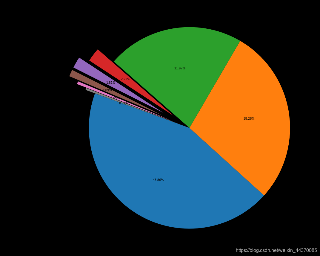
接下来我们首先看一下所有大类的paper数量分布:
我们使用merge函数,以两个dataframe共同的属性 “categories” 进行合并,并以 “group_name” 作为类别进行统计,统计结果放入 “id” 列中并排序。
_df = data.merge(df_taxonomy, on="categories", how="left").drop_duplicates(["id","group_name"]).groupby("group_name").agg({"id":"count"}).sort_values(by="id",ascending=False).reset_index()

_df
 	group_name 	id
0 	Physics 	79985
1 	Mathematics 	51567
2 	Computer Science 	40067
3 	Statistics 	4054
4 	Electrical Engineering and Systems Science 	3297
5 	Quantitative Biology 	1994
6 	Quantitative Finance 	826
7 	Economics 	576
下面我们使用饼图进行上图结果的可视化:
fig = plt.figure(figsize=(15,12))
explode = (0, 0, 0, 0.2, 0.3, 0.3, 0.2, 0.1)
plt.pie(_df["id"],  labels=_df["group_name"], autopct='%1.2f%%', startangle=160, explode=explode)
plt.tight_layout()
plt.show()
 下面统计在计算机各个子领域2019年后的paper数量,我们同样使用 merge 函数,对于两个dataframe 共同的特征 categories 进行合并并且进行查询。然后我们再对于数据进行统计和排序从而得到以下的结果:
group_name="Computer Science"
cats = data.merge(df_taxonomy, on="categories").query("group_name == @group_name")
cats.groupby(["year","category_name"]).count().reset_index().pivot(index="category_name", columns="year",values="id")
year 	2019 	2020
category_name
Artificial Intelligence 	558 	757
Computation and Language 	2153 	2906
Computational Complexity 	131 	188
Computational Engineering, Finance, and Science 	108 	205
Computational Geometry 	199 	216
Computer Science and Game Theory 	281 	323
Computer Vision and Pattern Recognition 	5559 	6517
Computers and Society 	346 	564
Cryptography and Security 	1067 	1238
Data Structures and Algorithms 	711 	902
Databases 	282 	342
Digital Libraries 	125 	157
Discrete Mathematics 	84 	81
Distributed, Parallel, and Cluster Computing 	715 	774
Emerging Technologies 	101 	84
Formal Languages and Automata Theory 	152 	137
General Literature 	5 	5
Graphics 	116 	151
Hardware Architecture 	95 	159
Human-Computer Interaction 	420 	580
Information Retrieval 	245 	331
Logic in Computer Science 	470 	504
Machine Learning 	177 	538
Mathematical Software 	27 	45
Multiagent Systems 	85 	90
Multimedia 	76 	66
Networking and Internet Architecture 	864 	783
Neural and Evolutionary Computing 	235 	279
Numerical Analysis 	40 	11
Operating Systems 	36 	33
Other Computer Science 	67 	69
Performance 	45 	51
Programming Languages 	268 	294
Robotics 	917 	1298
Social and Information Networks 	202 	325
Software Engineering 	659 	804
Sound 	7 	4
Symbolic Computation 	44 	36
Systems and Control 	415 	133


 被折叠的 条评论
为什么被折叠?
被折叠的 条评论
为什么被折叠?
 到【灌水乐园】发言


