


 本文展示了如何使用R语言读取CSV文件并进行初步的数据分析,包括统计和绘制交互式图表。首先通过`read.table`函数导入数据,接着计算不同条件下长度的平均值,再利用`aggregate`函数按类别分组求平均。最后,通过`interaction.plot`函数创建交互式图形,以直观对比不同条件下的数据分布。
> df<-read.table("工作簿1.csv",sep=",",header = T)
> df
读取数据
df<-read.table(“工作簿1.csv”,sep=",",header = T)
df
X len sup dose
1 1 7.4 wc 0.5
2 2 9.5 wc 0.5
3 3 3.4 wc 0.5
4 4 1.2 wc 1.0
5 5 8.3 wc 1.0
6 6 8.6 wc 1.0
7 7 5.3 wc 2.0
8 8 7.3 wc 2.0
9 9 8.5 wc 2.0
10 10 4.4 wc 2.0
11 11 8.1 oj 0.5
12 12 6.7 oj 0.5
13 13 3.7 oj 0.5
14 14 4.8 oj 1.0
15 15 0.6 oj 1.0
16 16 6.0 oj 1.0
17 17 0.9 oj 2.0
18 18 8.0 oj 2.0
19 19 3.7 oj 2.0
20 20 5.1 oj 2.0
统计值
table(df$ s u p , d f sup,df sup,dfdose)
0.5 1 2
oj 3 3 4
wc 3 3 4
求平均值:得出每种试验下均值的比较
aggregate(df$ l e n , b y = l i s t ( d f len,by=list(df len,by=list(dfsup,df$dose),FUN=mean)
Group.1 Group.2 x
1 oj 0.5 6.166667
2 wc 0.5 6.766667
3 oj 1.0 3.800000
4 wc 1.0 6.033333
5 oj 2.0 4.425000
6 wc 2.0 6.375000
求方差:每种试验下方差的比较:
aggregate(df$len,by=list(df$sup,df$dose),FUN=sd)
  Group.1 Group.2        x
1      oj     0.5 2.247962
2      wc     0.5 3.098925
3      oj     1.0 2.835489
4      wc     1.0 4.188476
5      oj     2.0 2.954516
6      wc     2.0 1.864359
使用aov进行方差均值
首先将计量的变量转换为分类变量因子factor,后面才可以进行1 2 分类
> class(df$dose)
[1] "numeric"
> df$dose<-as.factor(df$dose)
> class(df$dose)
[1] "factor"
接下来使用方差分析的函数aov进行数据分析
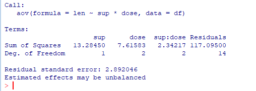
> fit<-aov(len~ sup*dose,data=df)
> fit
使用summary函数统计结果
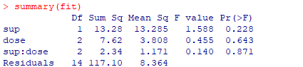
Pr(>F)这一项小于一定值表示非常显著
接下来用interact进行绘图
library(HH)
interaction.plot(df d o s e , d f dose,df dose,dfsup,df$len,type=“b”,col=c(“red”,“blue”),pch=c(16,18))


 被折叠的 条评论
为什么被折叠?
被折叠的 条评论
为什么被折叠?
 到【灌水乐园】发言


