第J5周：DenseNet+SE-Net实战（pytorch版）

本文链接：https://blog.youkuaiyun.com/weixin_43414521/article/details/142359845

>- **🍨 本文为[🔗365天深度学习训练营]中的学习记录博客**
>- **🍖 原作者：[K同学啊]**

本人往期文章可查阅：深度学习总结

📌 本周任务：
●1. 在DenseNet系列算法中插入SE-Net通道注意力机制，并完成猴痘病识别
●2. 改进思路是否可以迁移到其他地方呢
●3. 测试集accuracy到达89%（拔高，可选）

🏡 我的环境：

语言环境：Python3.8

编译器：Jupyter Notebook

深度学习环境：Pytorch

- torch==2.3.1+cu118

- torchvision==0.18.1+cu118

一、模型介绍

论文： Squeeze-and-Excitation Networks

SE-Net是ImageNet 2017 (lmageNet 收官赛)的冠军模型，是由自动驾驶公司Momenta在2017年公布的一种全新的图像识别结构，它通过对特征通道间的相关性进行建模，把重要的特征进行强化来提升准确率。这个结构是2017 ILSVR竞赛的冠军，top5的错误率达到了2.251%，比2016年的第一名还要低25%，可谓提升巨大。

模型具有复杂度低，参数少和计算量小的优点。且SENet 思路很简单，很容易扩展到已有网络结构如 Inception 和 ResNet 中。已经有很多工作在空间维度上来提升网络的性能，如 nception 等，而 SENet 将关注点放在了特征通道之间的关系上。其具体策略为: 通过学习的方式来自动获取到每个特征通道的重要程度，然后依照这个重要程度去提升有用的特征并抑制对当前任务用处不大的特征，这又叫做“特征重标定”策略。

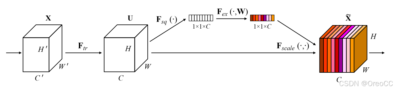
图1：SENet网络结构

给定一个输入 $x$ ，其特征通道数为 $c_{1}$ ，经过一系列卷积等一般变换 $F_{tr}$ ，后得到一个特征通道数为 $c_{2}$ 的特征。与传统的卷积神经网络不同，我们需要通过下面三个操作来重新标定前面得到的特征。

1.Squeeze

首先是Squeeze操作，我们顺着空间维度来进行特征压缩，将一个通道数和输入的特征通道数相等，例如可以将将形状为(1, 32, 32, 10)的feature map压缩成(1, 1, 1, 10)。此操作通常采用global average pooling来实现。也就是通过求每个通道 $c,c\in \left \{ 1,C \right \}$ 的Feature Map的平均值：

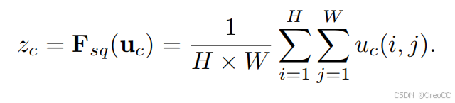
通过GAP得到的特征值是全局的（虽然比较粗糙）。另外， $z_{c}$ 也可以通过其它方法得到，要求只有一个，得到的特征向量具有全局性。

2.Excitation

得到了全局描述特征后，我们进行Excitation操作来抓取特征通道之间的关系。Excitation部分的作用是通过 $z_{c}$ 学习 $C$ 中每个通道的特征权值，要求有三点：

（1）要足够灵活，这样能保证学习到的权值比较具有价值；

（2）要足够简单，这样不至于添加SE blocks之后网络的训练速度大幅降低；

（3）通道之间的关系是non-exclusive的，也就是说学习到的特征能够激励重要的特征，抑制不重要的特征。

根据上面的要求，SE blocks使用了两层全连接构成的门机制（gate mechanism）。门控单元s（即图1中1x1xC的特征向量）的计算方式表示为：

$s=F_{ex}\left ( z,W\right )=\sigma \left ( g\left ( z,W \right ) \right )=\sigma \left ( W_{2}\delta \left ( W_{1}z \right ) \right )$

其中 $\delta$ 表示ReLU激活函数， $\sigma$ 表示sigmoid函数。 $W_{1}\in R^{\frac{C}{r}\times C}$ ， $W_{2}\in R^{C\times \frac{C}{r}}$ 分别是两个全连接层的权值矩阵。 $r$ 则是中间层的隐层节点数，论文中指出这个值是16.

这里采用包含两个全连接层的bottleneck结构，即中间小两头大的结构：其中第一个全链接层起到即降维的作用，并通过ReLU激活，第二个全链接层用来将其恢复至原始的维度。进行Excitation操作的最终目的是为每个特征通道生成权重，即学习到的各个通道的激活值（sigmoid激活，值在0~1之间）。
最后一个是Scale的操作，我们将Excitation的输出的权重看作是经过特征选择后的每个特征通道的重要性，然后通过乘法逐通道加权到先前的特征上，完成在通道维度上的对原始特征的重标定，从而提高了每一个通道在模型上的特征更有辨别能力,这类似于attention机制。

二、SE模块应用分析

SE模块非常灵活,表现在其可以直接应用在现有的网络结果中,以Inception和ResNet为例,左侧是SE-Inception的结构，即Inception模块和SENet组和在一起；右侧是SE-ResNet，ResNet和SENet的组合，这种结构scale放到了直连相加之前。

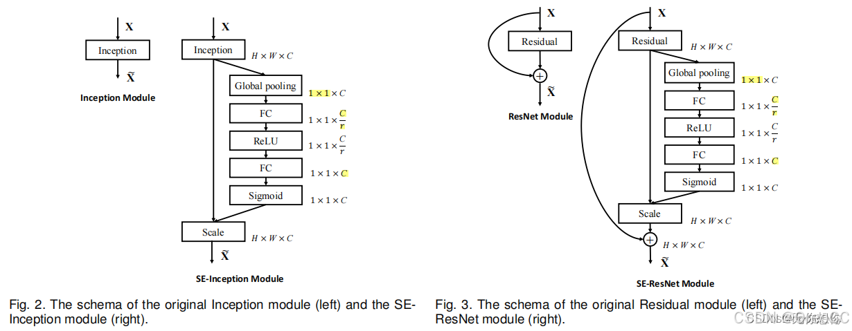
方框旁边的维度信息代表该层的输出， $r$ 表示Excitation(激发)操作当中的降维系数。

三、SE模块的效果对比

1、ImageNet测试

SE模块很容易嵌入到其他网络中，为了验证SE模块的作用，在其他流行网络如ResNet和Inception中引入SE模块，测试其在ImageNet上的效果，如下表所示：

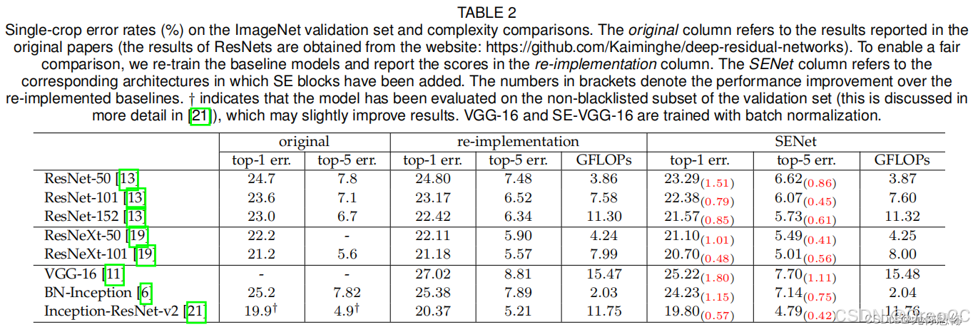
首先看一下网络的深度对SE的影响。上表分别展示了ResNet-50、ResNet-101、ResNet-152和嵌入SE模型的结果。第一栏Original是原作者实现的结果，为了进行公平的比较，重新进行了实验得到Our re-implementation的结果。最后一栏SE-module是指嵌入了SE模块的结果，它的训练参数和第二栏Our re-implementation一致。括号中的红色数值是指相对于Our re-implementation的精度提升的幅值。

从上表可以看出，SE-ResNets在各种深度上都远远超过了其对应的没有SE的结构版本的精度,这表示无论网络的深度以及大小，SE模块都能够给网络带来性能上的增益。值得一提的是，SE-ResNet-50可以达到和ResNet-101一样的精度；更甚，SE-ResNet-101远远地超过了更深的ResNet-152

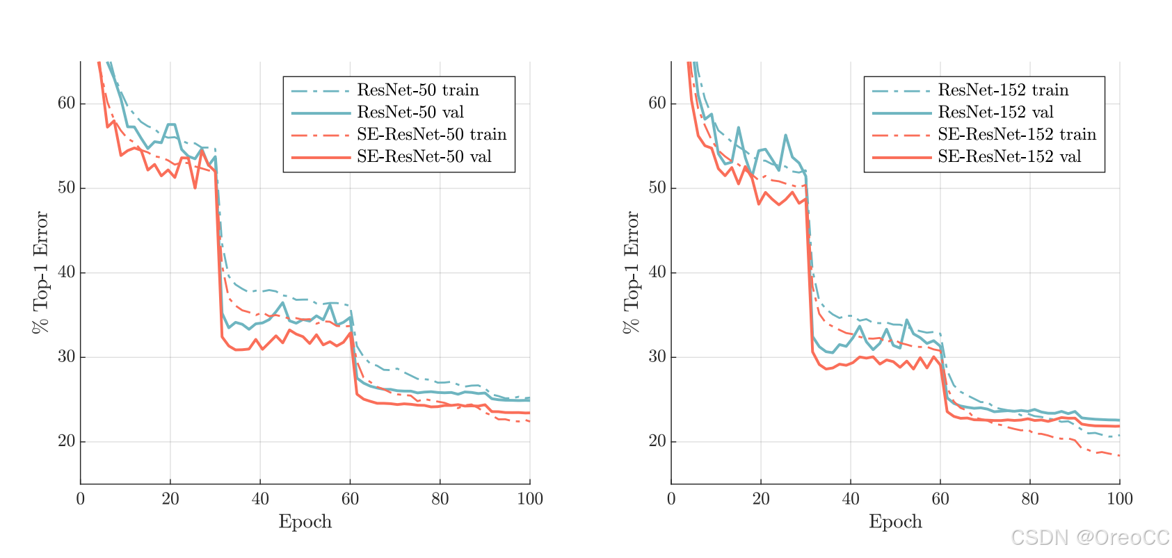
上图展示了ResNet-50和ResNet-152以及他们对应的嵌入SE模块的网络在ImageNet上的训练过程，可以明显地看出加入了SE模块的网络收敛到更低的错误率上。

2、场景分类测试

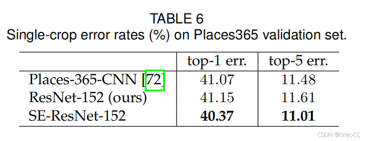
作者用Place365数据集进行了场景分类测试，比较的结构是ResNet-152和SE-ResNet-152，结果见图7，可以看出SENet在ImageNet以外的数据集上仍有优势。

四、前期准备

1、设置GPU

import warnings
warnings.filterwarnings("ignore") #忽略警告信息

import torch
device=torch.device("cuda" if torch.cuda.is_available() else "CPU")
device

运行结果：

device(type='cuda')

2、导入数据

import pathlib

data_dir=r'D:\THE MNIST DATABASE\P4-data'
data_dir=pathlib.Path(data_dir)

image_count=len(list(data_dir.glob('*/*')))
print("图片总数为：",image_count)

运行结果：

图片总数为： 2142

3、查看数据集分类

data_paths=list(data_dir.glob('*'))
classeNames=[str(path).split("\\")[3] for path in data_paths]
classeNames

运行结果：

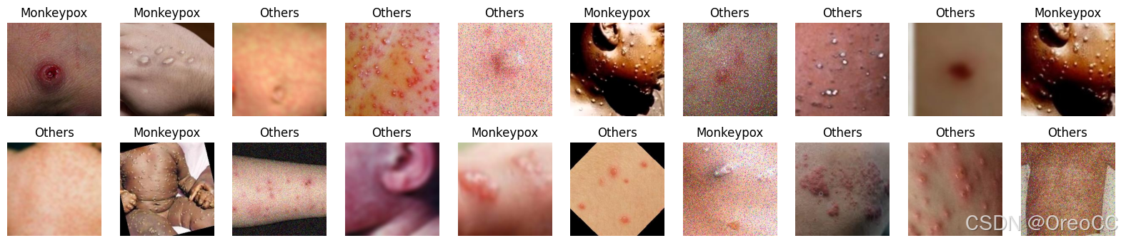
['Monkeypox', 'Others']

4、随机查看图片

随机抽取数据集中的20张图片进行查看

import random,PIL
import matplotlib.pyplot as plt
from PIL import Image

data_paths2=list(data_dir.glob('*/*'))
plt.figure(figsize=(20,4))
for i in range(20):
    plt.subplot(2,10,i+1)
    plt.axis('off')
    image=random.choice(data_paths2) #随机选择一张图片
    plt.title(image.parts[-2]) #通过glob对象取出他的文件夹名称，即分类名
    plt.imshow(Image.open(str(image))) #显示图片

运行结果：

5、图片预处理

import torchvision.transforms as transforms
from torchvision import transforms,datasets

train_transforms=transforms.Compose([
    transforms.Resize([224,224]), #将图片统一尺寸
    transforms.RandomHorizontalFlip(), #将图片随机水平翻转
    transforms.RandomRotation(0.2), #将图片按照0.2弧度值随机翻转
    transforms.ToTensor(), #将图片转换为tensor
    transforms.Normalize(  #标准化处理-->转换为正太分布，使模型更容易收敛
        mean=[0.485,0.456,0.406],
        std=[0.229,0.224,0.225]
    )
])

total_data=datasets.ImageFolder(
    r'D:\THE MNIST DATABASE\P4-data',
    transform=train_transforms
)
total_data

运行结果：

Dataset ImageFolder
    Number of datapoints: 2142
    Root location: D:\THE MNIST DATABASE\P4-data
    StandardTransform
Transform: Compose(
               Resize(size=[224, 224], interpolation=bilinear, max_size=None, antialias=True)
               RandomHorizontalFlip(p=0.5)
               RandomRotation(degrees=[-0.2, 0.2], interpolation=nearest, expand=False, fill=0)
               ToTensor()
               Normalize(mean=[0.485, 0.456, 0.406], std=[0.229, 0.224, 0.225])
           )

将数据集分类情况进行映射输出：

total_data.class_to_idx

运行结果：

{'Monkeypox': 0, 'Others': 1}

6、划分数据集

train_size=int(0.8*len(total_data))
test_size=len(total_data)-train_size
train_size,test_size

运行结果：

(1713, 429)

train_dataset,test_dataset=torch.utils.data.random_split(
    total_data,
    [train_size,test_size]
)
train_dataset,test_dataset

运行结果：

(<torch.utils.data.dataset.Subset at 0x234f4a59c10>,
 <torch.utils.data.dataset.Subset at 0x234f4a58050>)

7、加载数据集

batch_size=16
train_dl=torch.utils.data.DataLoader(
    train_dataset,
    batch_size=batch_size,
    shuffle=True,
    num_workers=1
)
test_dl=torch.utils.data.DataLoader(
    test_dataset,
    batch_size=batch_size,
    shuffle=True,
    num_workers=1
)

查看测试集的情况：

for x,y in train_dl:
    print("Shape of x [N,C,H,W]:",x.shape)
    print("Shape of y:",y.shape,y.dtype)
    break

运行结果：

Shape of x [N,C,H,W]: torch.Size([16, 3, 224, 224])
Shape of y: torch.Size([16]) torch.int64

五、手动搭建DenseNet+SE-Net模型

1、SE模块实现

import torch.nn as nn
import torch.nn.functional as F

''' Squeeze Excitation Module '''
class SEModule(nn.Module):
    def __init__(self, in_channel, filter_sq=16):
        super(SEModule, self).__init__()
        self.se = nn.Sequential(
            nn.AdaptiveAvgPool2d((1, 1)),
            nn.Flatten(),
            nn.Linear(in_channel, in_channel//filter_sq),
            nn.ReLU(True),
            nn.Linear(in_channel//filter_sq, in_channel),
            nn.Sigmoid()
        )
        #self.se = nn.Sequential(
        #    nn.AdaptiveAvgPool2d((1,1)),
        #    nn.Conv2d(in_channel, in_channel//filter_sq, kernel_size=1),
        #    nn.ReLU(),
        #    nn.Conv2d(in_channel//filter_sq, in_channel, kernel_size=1),
        #    nn.Sigmoid()
        #)
    
    def forward(self, inputs):
        x = self.se(inputs)
        s1, s2 = x.size(0), x.size(1)
        x = torch.reshape(x, (s1, s2, 1, 1))
        x = inputs * x
        return x

2、在DenseNet中添加SE模块

实现DenseBlock模块和Transition层：

''' Basic unit of DenseBlock (using bottleneck layer) '''
class DenseLayer(nn.Sequential):
    def __init__(self, in_channel, growth_rate, bn_size, drop_rate):
        super(DenseLayer, self).__init__()
        self.add_module('norm1', nn.BatchNorm2d(in_channel))
        self.add_module('relu1', nn.ReLU(inplace=True))
        self.add_module('conv1', nn.Conv2d(in_channel, bn_size*growth_rate,
                                           kernel_size=1, stride=1, bias=False))
        self.add_module('norm2', nn.BatchNorm2d(bn_size*growth_rate))
        self.add_module('relu2', nn.ReLU(inplace=True))
        self.add_module('conv2', nn.Conv2d(bn_size*growth_rate, growth_rate,
                                           kernel_size=3, stride=1, padding=1, bias=False))
        self.drop_rate = drop_rate
    
    def forward(self, x):
        new_feature = super(DenseLayer, self).forward(x)
        if self.drop_rate>0:
            new_feature = F.dropout(new_feature, p=self.drop_rate, training=self.training)
        return torch.cat([x, new_feature], 1)
 
 
''' DenseBlock '''
class DenseBlock(nn.Sequential):
    def __init__(self, num_layers, in_channel, bn_size, growth_rate, drop_rate):
        super(DenseBlock, self).__init__()
        for i in range(num_layers):
            layer = DenseLayer(in_channel+i*growth_rate, growth_rate, bn_size, drop_rate)
            self.add_module('denselayer%d'%(i+1,), layer)
 
 
''' Transition layer between two adjacent DenseBlock '''
class Transition(nn.Sequential):
    def __init__(self, in_channel, out_channel):
        super(Transition, self).__init__()
        self.add_module('norm', nn.BatchNorm2d(in_channel))
        self.add_module('relu', nn.ReLU(inplace=True))
        self.add_module('conv', nn.Conv2d(in_channel, out_channel,
                                          kernel_size=1, stride=1, bias=False))
        self.add_module('pool', nn.AvgPool2d(2, stride=2))

实现DenseNet-SE 网络：

from collections import OrderedDict
import torch.utils.checkpoint as cp


''' DenseNet-BC model '''
class DenseNet(nn.Module):
    def __init__(self, growth_rate=32, block_config=(6,12,24,16), init_channel=64, 
                 bn_size=4, compression_rate=0.5, drop_rate=0, num_classes=1000):
        '''
        :param growth_rate: (int) number of filters used in DenseLayer, `k` in the paper
        :param block_config: (list of 4 ints) number of layers in eatch DenseBlock
        :param init_channel: (int) number of filters in the first Conv2d
        :param bn_size: (int) the factor using in the bottleneck layer
        :param compression_rate: (float) the compression rate used in Transition Layer
        :param drop_rate: (float) the drop rate after each DenseLayer
        :param num_classes: (int) number of classes for classification
        '''
        super(DenseNet, self).__init__()
        # first Conv2d
        self.features = nn.Sequential(OrderedDict([
            ('conv0', nn.Conv2d(3, init_channel, kernel_size=7, stride=2, padding=3, bias=False)),
            ('norm0', nn.BatchNorm2d(init_channel)),
            ('relu0', nn.ReLU(inplace=True)),
            ('pool0', nn.MaxPool2d(3, stride=2, padding=1))
        ]))
        # DenseBlock
        num_features = init_channel
        for i, num_layers in enumerate(block_config):
            block = DenseBlock(num_layers, num_features, bn_size, growth_rate, drop_rate)
            self.features.add_module('denseblock%d'%(i+1), block)
            num_features += num_layers*growth_rate
            if i!=len(block_config)-1:
                transition = Transition(num_features, int(num_features*compression_rate))
                self.features.add_module('transition%d'%(i+1), transition)
                num_features = int(num_features*compression_rate)
        # SE Module
        self.features.add_module('SE-module', SEModule(num_features))
        # final BN+ReLU
        self.features.add_module('norm5', nn.BatchNorm2d(num_features))
        self.features.add_module('relu5', nn.ReLU(inplace=True))
        # classification layer
        self.classifier = nn.Linear(num_features, num_classes)
        # params initialization
        for m in self.modules():
            if isinstance(m, nn.Conv2d):
                nn.init.kaiming_normal_(m.weight)
            elif isinstance(m, nn.BatchNorm2d):
                nn.init.constant_(m.bias, 0)
                nn.init.constant_(m.weight