Tensorflow小白实战系列

一、环境需要

tensorflow-CPU版本
jupyter
python3
MNIST_data(MNIST数据集)

二、卷积神经网络的结构

Mnist数据集中，每一张图片都是（28，28，1），即图片的宽高都是28，通道数为1，代表这是灰度图片。我们将要讲解并实现一个系列的教程，用不同的API来搭建卷积神经网络，今天我们来进入第一种搭建的方法----自定义卷积核池化函数，然后调用函数完成网络的搭建。
输入的图像是（28，28，1）
第一个卷积层：16个55的卷积核
输出：141416
第二个卷积层：36个55的卷积核
输出：7736
resize操作：送入全连接之前将图片展平成（None,7736）
第一个全连接层：128
第二个全连接层：10

三、数据集的导入与可视化

1.1导入相应的模块

import matplotlib.pyplot as plt
import tensorflow as tf
import numpy as np
from sklearn.metrics import confusion_matrix
import time
from datetime import timedelta
import math

1.2 导入数据集

from tensorflow.examples.tutorials.mnist import input_data
data = input_data.read_data_sets(r'C:\Users\满森\项目\deep_learning\MNIST_data/', one_hot=True)

1.3 设置图片的大小尺寸

# The number of pixels in each dimension of an image.
img_size = 28
# The images are stored in one-dimensional arrays of this length.
img_size_flat = 28*28
# Tuple with height and width of images used to reshape arrays.
img_shape = (28,28)
# Number of classes, one class for each of 10 digits.
num_classes = 10
# Number of colour channels for the images: 1 channel for gray-scale.
num_channels = 1

1.4 定义函数，绘制图片

def plot_images(images, cls_true, cls_pred=None):
    assert len(images) == len(cls_true) == 9
    
    # Create figure with 3x3 sub-plots.
    fig, axes = plt.subplots(3, 3)
    fig.subplots_adjust(hspace=0.3, wspace=0.3)

    for i, ax in enumerate(axes.flat):
        # Plot image.
        ax.imshow(images[i].reshape(img_shape), cmap='binary')

        # Show true and predicted classes.
        if cls_pred is None:
            xlabel = "True: {0}".format(cls_true[i])
        else:
            xlabel = "True: {0}, Pred: {1}".format(cls_true[i], cls_pred[i])

        # Show the classes as the label on the x-axis.
        ax.set_xlabel(xlabel)
        
        # Remove ticks from the plot.
        ax.set_xticks([])
        ax.set_yticks([])
    
    # Ensure the plot is shown correctly with multiple plots
    # in a single Notebook cell.
    plt.show()

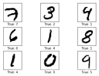
1.5 绘制几张图片

# Get the first images from the test-set.
images = data.train.images[0:9]

# Get the true classes for those images.
cls_true = np.argmax(data.test.labels[0:9],axis=1)

# Plot the images and labels using our helper-function above.
plot_images(images=images, cls_true=cls_true)

四、网络搭建的辅助函数

1.1 定义帮助函数
（1）权重初始化

def new_weights(shape):
    return tf.Variable(tf.truncated_normal(shape, stddev=0.05))

（2）偏置初始化

def new_biases(length):
    return tf.Variable(tf.constant(0.05, shape=[length]))

（3）定义卷积操作

def new_conv_layer(input,              # The previous layer.
                   num_input_channels, # Num. channels in prev. layer.
                   filter_size,        # Width and height of each filter.
                   num_filters,        # Number of filters.
                   use_pooling=True):  # Use 2x2 max-pooling.

    shape = [filter_size, filter_size, num_input_channels, num_filters]

    weights = new_weights(shape=shape)

    biases = new_biases(length=num_filters)

    layer = tf.nn.conv2d(input=input,
                         filter=weights,
                         strides=[1, 1, 1, 1],
                         padding='SAME')

    layer += biases

	# 判断是否使用池化，池化核2*2，步长2
	# 池化之后图像尺寸变小
    if use_pooling:
        layer = tf.nn.max_pool(value=layer,
                               ksize=[1, 2, 2, 1],
                               strides=[1, 2, 2, 1],
                               padding='SAME')
	# 池化之后送给非线性
    layer = tf.nn.relu(layer)
	# 返回非线性输出和权重
    return layer, weights

（4）送入全连接层之前将向量展平

def flatten_layer(layer):
    # Get the shape of the input layer.
    layer_shape = layer.get_shape()
    num_features = layer_shape[1:4].num_elements()
    layer_flat = tf.reshape(layer, [-1, num_features])
    return layer_flat, num_features

（5）定义全连接操作

def new_fc_layer(input,          # The previous layer.
                 num_inputs,     # Num. inputs from prev. layer.
                 num_outputs,    # Num. outputs.
                 use_relu=True): # Use Rectified Linear Unit (ReLU)?

    # Create new weights and biases.
    weights = new_weights(shape=[num_inputs, num_outputs])
    biases = new_biases(length=num_outputs)

    # Calculate the layer as the matrix multiplication of
    # the input and weights, and then add the bias-values.
    layer = tf.matmul(input, weights) + biases

    # Use ReLU?
    if use_relu:
        layer = tf.nn.relu(layer)

    return layer

五、搭建卷积神经网络

（1）设置占位符

x = tf.placeholder(tf.float32, shape=[None, img_size_flat], name='x')
x_image = tf.reshape(x, [-1, img_size, img_size, num_channels])
y_true = tf.placeholder(tf.float32, shape=[None, num_classes], name='y_true')
y_true_cls = tf.argmax(y_true, axis=1)

（2）第一个卷积层

layer_conv1, weights_conv1 = \
    new_conv_layer(input=x_image,
                   num_input_channels=num_channels,
                   filter_size=filter_size1,
                   num_filters=num_filters1,
                   use_pooling=True)

（3）第二个卷积层

layer_conv2, weights_conv2 = \
    new_conv_layer(input=layer_conv1,
                   num_input_channels=num_filters1,
                   filter_size=filter_size2,
                   num_filters=num_filters2,
                   use_pooling=True)

（4）第一个全连接层

## 首先将向量展平
layer_flat, num_features = flatten_layer(layer_conv2)
## 然后送入全连接层
layer_fc1 = new_fc_layer(input=layer_flat,
                         num_inputs=num_features,
                         num_outputs=fc_size,
                         use_relu=True)

（5）第二个全连接层

layer_fc2 = new_fc_layer(input=layer_fc1,
                         num_inputs=fc_size,
                         num_outputs=num_classes,
                         use_relu=False)

（6）损失函数与优化

# 将输出层送入softmax，结果是预测的十个标签对应的得分（0-1）
y_pred = tf.nn.softmax(layer_fc2)
# 每一行求argmax，得到其正确分类
y_pred_cls = tf.argmax(y_pred, axis=1)
# 交叉熵损失函数
cross_entropy =tf.nn.softmax_cross_entropy_with_logits(logits=layer_fc2,
                                        labels=y_true)
# 求均值之后即为损失函数
cost = tf.reduce_mean(cross_entropy)
# 定义优化器，优化损失函数
optimizer = tf.train.AdamOptimizer(learning_rate=1e-4).minimize(cost)
# 得到正确率，即预测标签和正确标签作对比
correct_prediction = tf.equal(y_pred_cls, y_true_cls)
accuracy = tf.reduce_mean(tf.cast(correct_prediction, tf.float32))

（7）开启会话，全局初始化
经过上面的过程，我们的卷积神经网络已将搭建成功。但是我们没有喂入数据，在进行这些操作之前，我们要开启会话，这和Tensorflow 的运行机制有关，记住一切的计算都要在会话中进行。

session = tf.Session()
session.run(tf.global_variables_initializer())

六、进行优化，结果展示辅助函数

（1）定义优化器
我们按照一个batch 进行训练，这样可以加快速度，每一轮训练64张图片

train_batch_size = 64
total_iterations = 0
def optimize(num_iterations):
    # Ensure we update the global variable rather than a local copy.
    global total_iterations

    # Start-time used for printing time-usage below.
    start_time = time.time()

    for i in range(total_iterations,
                   total_iterations + num_iterations):

        # Get a batch of training examples.
        # x_batch now holds a batch of images and
        # y_true_batch are the true labels for those images.
        x_batch, y_true_batch = data.train.next_batch(train_batch_size)

        # Put the batch into a dict with the proper names
        # for placeholder variables in the TensorFlow graph.
        feed_dict_train = {x: x_batch,
                           y_true: y_true_batch}

        # Run the optimizer using this batch of training data.
        # TensorFlow assigns the variables in feed_dict_train
        # to the placeholder variables and then runs the optimizer.
        session.run(optimizer, feed_dict=feed_dict_train)

        # Print status every 100 iterations.
        if i % 100 == 0:
            # Calculate the accuracy on the training-set.
            acc = session.run(accuracy, feed_dict=feed_dict_train)

            # Message for printing.
            msg = "Optimization Iteration: {0:>6}, Training Accuracy: {1:>6.1%}"

            # Print it.
            print(msg.format(i + 1, acc))

    # Update the total number of iterations performed.
    total_iterations += num_iterations

    # Ending time.
    end_time = time.time()

    # Difference between start and end-times.
    time_dif = end_time - start_time

    # Print the time-usage.
    print("Time usage: " + str(timedelta(seconds=int(round(time_dif)))))

（2）绘制错误图片
cls_true = data.test.labels
cls_true = np.argmax(cls_true,axis = 1)
这两句话的意思是我们得到标签确切的分类

def plot_example_errors(cls_pred, correct):


    incorrect = (correct == False)
    # 找到错误图片
    images = data.test.images[incorrect].
    # 得到错误分类标签
    cls_pred = cls_pred[incorrect]
    # 得到真实标签
    cls_true = data.test.labels
    cls_true = np.argmax(cls_true,axis = 1)
    cls_true = cls_true[incorrect]
    
    # Plot the first 9 images.
    plot_images(images=images[0:9],
                cls_true=cls_true[0:9],
                cls_pred=cls_pred[0:9])

（3）绘制混淆矩阵

def plot_confusion_matrix(cls_pred):
    # This is called from print_test_accuracy() below.
    cls_true = data.test.labels
    cls_true = np.argmax(cls_true,axis = 1) 
    # Get the confusion matrix using sklearn.
    cm = confusion_matrix(y_true=cls_true,
                          y_pred=cls_pred)
    # Print the confusion matrix as text.
    print(cm)
    # Plot the confusion matrix as an image.
    plt.matshow(cm)
    # Make various adjustments to the plot.
    plt.colorbar()
    tick_marks = np.arange(num_classes)
    plt.xticks(tick_marks, range(num_classes))
    plt.yticks(tick_marks, range(num_classes))
    plt.xlabel('Predicted')
    plt.ylabel('True')
    plt.show()

（4）定义函数，打印测试集准确率

# Split the test-set into smaller batches of this size.
test_batch_size = 256

def print_test_accuracy(show_example_errors=False,
                        show_confusion_matrix=False):
    num_test = len(data.test.images)
    cls_pred = np.zeros(shape=num_test, dtype=np.int)

    i = 0

    while i < num_test:
        # The ending index for the next batch is denoted j.
        j = min(i + test_batch_size, num_test)

        # Get the images from the test-set between index i and j.
        images = data.test.images[i:j, :]

        # Get the associated labels.
        labels = data.test.labels[i:j, :]

        # Create a feed-dict with these images and labels.
        feed_dict = {x: images,
                     y_true: labels}

        # Calculate the predicted class using TensorFlow.
        cls_pred[i:j] = session.run(y_pred_cls, feed_dict=feed_dict)

        # Set the start-index for the next batch to the
        # end-index of the current batch.
        i = j
    cls_true = data.test.labels
    cls_true = np.argmax(cls_true,axis=1)
    correct = np.float32((cls_true == cls_pred))
    correct_sum = correct.sum()
    acc = float(correct_sum) / num_test

    # Print the accuracy.
    msg = "Accuracy on Test-Set: {0:.1%} ({1} / {2})"
    print(msg.format(acc, correct_sum, num_test))

    # Plot some examples of mis-classifications, if desired.
    if show_example_errors:
        print("Example errors:")
        plot_example_errors(cls_pred=cls_pred, correct=correct)

    # Plot the confusion matrix, if desired.
    if show_confusion_matrix:
        print("Confusion Matrix:")
        plot_confusion_matrix(cls_pred=cls_pred)

七、结果显示

（1）优化1000次

optimize(num_iterations=900) # We performed 100 iterations above.

Optimization Iteration:    201, Training Accuracy:  81.2%
Optimization Iteration:    301, Training Accuracy:  87.5%
Optimization Iteration:    401, Training Accuracy:  87.5%
Optimization Iteration:    501, Training Accuracy:  96.9%
Optimization Iteration:    601, Training Accuracy:  87.5%
Optimization Iteration:    701, Training Accuracy:  95.3%
Optimization Iteration:    801, Training Accuracy:  90.6%
Optimization Iteration:    901, Training Accuracy:  93.8%
Optimization Iteration:   1001, Training Accuracy:  96.9%
Time usage: 0:00:40

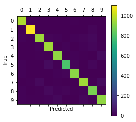
（2）打印结果并展示混淆矩阵

print_test_accuracy(show_confusion_matrix=True)

Accuracy on Test-Set: 93.4% (9341.0 / 10000)
Confusion Matrix:
[[ 968    0    0    1    0    1    5    1    4    0]
 [   0 1105    4    3    1    1    4    0   17    0]
 [  10    1  945   17   11    0    9   13   25    1]
 [   2    3    9  949    0   10    1   11   19    6]
 [   1    1    6    1  921    0   11    5    3   33]
 [  12    2    3   33    8  791   17    1   21    4]
 [  12    3    3    1   10   13  912    1    3    0]
 [   0    5   28    4    5    0    0  947    5   34]
 [   9    0    6   26   10   15    5   12  883    8]
 [   9    5    7   12   25    4    0   19    8  920]]

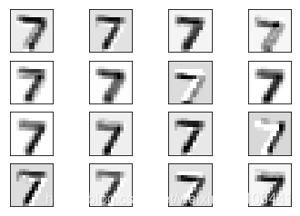
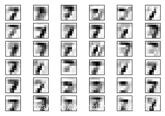
八，卷积输出可视化

（1）绘制帮助函数

def plot_conv_layer(layer, image):

    feed_dict = {x: [image]}

    values = session.run(layer, feed_dict=feed_dict)

    num_filters = values.shape[3]

    num_grids = math.ceil(math.sqrt(num_filters))
    
    # Create figure with a grid of sub-plots.
    fig, axes = plt.subplots(num_grids, num_grids)

    # Plot the output images of all the filters.
    for i, ax in enumerate(axes.flat):
        # Only plot the images for valid filters.
        if i<num_filters:
            img = values[0, :, :, i]
            # Plot image.
            ax.imshow(img, interpolation='nearest', cmap='binary')   
        # Remove ticks from the plot.
        ax.set_xticks([])
        ax.set_yticks([])
    plt.show()

（2）绘制图片

image1 = data.test.images[0]
plot_conv_layer(layer=layer_conv1, image=image1)

plot_conv_layer(layer=layer_conv2, image=image1)