


 这是关于吴恩达机器学习课程的详细笔记,涵盖了监督学习、非监督学习、线性回归等内容。笔记中详细解释了如何使用梯度下降算法最小化代价函数,并通过实例演示了如何在Python中实现。
Machine Learning By Andrew Ng (吴恩达机器学习笔记 英文版)
这是我记录的吴恩达机器学习的课堂笔记。但是我记录的是英文版,所以如果有什么地方记录不准确,希望大家指出。另外,我也见到了中文版的笔记,但是只有第一章。学习了中文版后,我打算在学习ML之余,结合我自己的理解,不断更新这个笔记。
有人觉得ML很难,但是我要说明一点。作为XDU的大一学生,我在第一年的结束时,高数总评93期末98,线代总评96期末93分。在前三章的学习中,如果对这两门掌握很好,学起来并不是非常费劲的。
Machine Learning 101
Reguassion and Classification Problem
Reguassion vs Classification
Instance:
Reguassion predicts housing price.
Classification predicts discrete output like if have a tumor.
Octave for ML, or Matlab(java or c++ and python requires tons of code to do the same thing!)
Model Discription
m = number of training examples
x = input variable / feature
y = output or target variable
(x, y) = one training example
( x ( i ) , y ( i ) x^{(i)}, y^{(i)} x(i),y(i)) = the i t h i^{th} ith training example # i i i stands for index
Linear Regression
the simple one
![[外链图片转存失败(img-DUj2v4YY-1562145993382)(C:\Users\chenh\Desktop\Notebook\Machine Learing\2019-6-30.png)]](https://i-blog.csdnimg.cn/blog_migrate/afc860eee033f5d15bd2a500f54b8d77.png)
Hypothesis: h θ ( x ) = θ 0 + θ 1 x h_{\theta}(x) = \theta_0 + \theta_1x hθ(x)=θ0+θ1x
θ i \theta_i θi: Parameter
Univariate Cost Function
–How to choose different patameters, AKA θ 0 , θ 1 \theta_0, \theta_1 θ0,θ1?
We want the h θ h_{\theta} hθ fit the data (close to y y y) well, so we have to find the ideal θ 0 , θ 1 \theta_0, \theta_1 θ0,θ1, that make sure for every x ( i ) x^{(i)} x(i) in data example set:
→ h θ ( x ) − y \rightarrow h_\theta(x) - y →hθ(x)−y small enough,
→ ( h θ ( x ) − y ) 2 \rightarrow{(h_\theta(x) - y)}^2 →(hθ(x)−y)2 small enough,
finally,
→ 1 2 m ∑ i = 1 m ( h θ ( x ( i ) ) − y ( i ) ) 2 \rightarrow\frac{1}{2m}\sum_{i=1}^m{(h_\theta(x^{(i)}) - y^{(i)})}^2 →2m1∑i=1m(hθ(x(i))−y(i))2small enough.
To be clear, we define that latest function as :
J ( θ 0 , θ 1 ) = 1 2 m ∑ i = 1 m ( h θ ( x ( i ) ) − y ( i ) ) 2 J(\theta_0,\theta_1) = \frac{1}{2m}\sum_{i=1}^m{(h_\theta(x^{(i)}) - y^{(i)})}^2 J(θ0,θ1)=2m1∑i=1m(hθ(x(i))−y(i))2
Now the only thing we need to do is find the minimum of $J(\theta_0,\theta_1) $, so we call $J(\theta_0,\theta_1) $ as cost function or squared error function.
Now, for better understanding, we simplified h θ ( x ) = θ 1 x h_\theta(x) = \theta_1 x hθ(x)=θ1x, and our goal is minimize J ( 0 , θ 1 ) J(0, \theta_1) J(0,θ1)
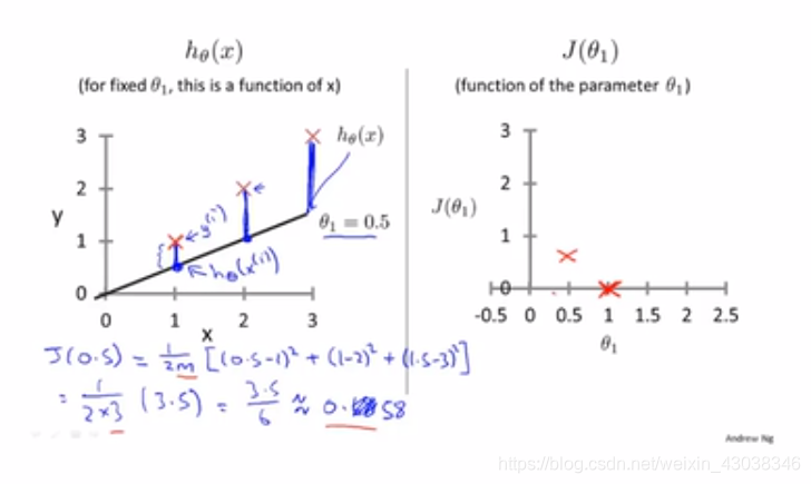
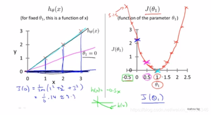
h θ ( x ) h_\theta(x) hθ(x) vs J ( θ 1 ) J(\theta_1) J(θ1)
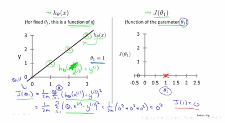
Now we find the perfect
θ
1
=
1
\theta_1 = 1
θ1=1
Back to J ( θ 0 , θ 1 ) J(\theta_0,\theta_1) J(θ0,θ1), whatever J ( θ 0 , θ 1 ) J(\theta_0,\theta_1) J(θ0,θ1) or J ( θ 0 ) J(\theta_0) J(θ0) we can plot a bowl shaped picture. But the difference is the dimension. To show J ( θ 0 , θ 1 ) J(\theta_0,\theta_1) J(θ0,θ1), we don’t have to draw 3D pic, so we use contour plots(等高线) to dipict J ( θ 0 , θ 1 ) J(\theta_0,\theta_1) J(θ0,θ1).
We want a software(algorithm) to find the ideal θ 0 , θ 1 \theta_0,\theta_1 θ0,θ1 automatically.
Gradient descent
for minimizing function J J J and so on.
Idea
- Start with some θ 0 , θ 1 \theta_0, \theta_1 θ0,θ1.
- Keep changing it to reduce J ( θ 0 , θ 1 ) J(\theta_0, \theta_1) J(θ0,θ1) until we end up at a minimum.
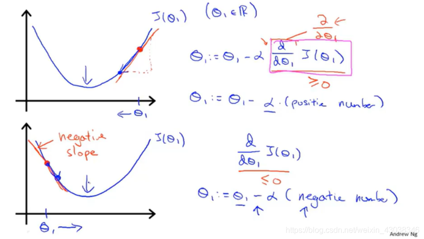
Gradient descent algorithm
repeat until convergence {
θ j : = θ j − α ∂ J ( θ 0 , θ 1 ) ∂ θ j \theta_j := \theta_j - \alpha \frac{\partial J(\theta_0, \theta_1) }{\partial \theta_j} θj:=θj−α∂θj∂J(θ0,θ1) (for j = 0 j = 0 j=0 and j = 1 j = 1 j=1)
}
α \alpha α: learning rate(how big thee step is)
This is an update equation, simultaneously update θ 0 \theta_0 θ0 and θ 1 \theta_1 θ1, which like the followings.
Corrent Update
t e m p 0 : = θ 0 − α ∂ J ( θ 0 , θ 1 ) ∂ θ 0 temp0 := \theta_0 - \alpha \frac{\partial J(\theta_0, \theta_1) }{\partial \theta_0} temp0:=θ0−α∂θ0∂J(θ0,θ1)
t e m p 1 : = θ 1 − α ∂ J ( θ 0 , θ 1 ) ∂ θ 1 temp1:= \theta_1 - \alpha \frac{\partial J(\theta_0, \theta_1) }{\partial \theta_1} temp1:=θ1−α∂θ1∂J(θ0,θ1)
θ 0 : = t e m p 0 \theta_0 := temp0 θ0:=temp0
θ 1 : = t e m p 1 \theta_1 := temp1 θ1:=temp1
Incorrent (does not refer to gradient descent algorithm)
t e m p 0 : = θ 0 − α ∂ J ( θ 0 , θ 1 ) ∂ θ 0 temp0 := \theta_0 - \alpha \frac{\partial J(\theta_0, \theta_1) }{\partial \theta_0} temp0:=θ0−α∂θ0∂J(θ0,θ1)
θ 0 : = t e m p 0 \theta_0 := temp0 θ0:=temp0
t e m p 1 : = θ 1 − α ∂ J ( θ 0 , θ 1 ) ∂ θ 1 temp1:= \theta_1 - \alpha \frac{\partial J(\theta_0, \theta_1) }{\partial \theta_1} temp1:=θ1−α∂θ1∂J(θ0,θ1) (new θ 0 \theta_0 θ0 in this step)
θ 1 = t e m p 1 \theta_1 = temp1 θ1=temp1
So, we have to define Variables like temp* to collect all the
θ
\theta
θ’ s.
The partial derivative term in the equation
The α \alpha α term in the equation
- If the α \alpha α is too small, the progress is slow.
- If it is too big, we may overshoot (miss) the minimum. It may fail to converge, or even diverge.
Q: What if your parameter θ 1 \theta_1 θ1 is already at the local minimum, what do you think one step of gradient descent (algorithm) will do?
A: θ 1 \theta_1 θ1 won’t change because the derivative term is equal to zero, that will keep θ 1 \theta_1 θ1 at the local optimum. (It is actually basic calculus. )
Gradient descent can converge to a local minimum, even with the learning rate α \alpha α fixed. As we approach a local minimum, gradient descent will automatically take smaller steps. So, no need to decrease α \alpha α over time.
You can use gradient descent algorithm to minimize any cost function J J J, not only defined for linear regression.
Gradient descent for linear regerssion
review
-
Linear Regression Model
J ( θ 0 , θ 1 ) = 1 2 m ∑ i = 1 m ( h θ ( x ( i ) ) − y ( i ) ) 2 J(\theta_0,\theta_1) = \frac{1}{2m}\sum_{i=1}^m{(h_\theta(x^{(i)}) - y^{(i)})}^2 J(θ0,θ1)=2m1∑i=1m(hθ(x(i))−y(i))2
h θ ( x ) = θ 0 + θ 1 x h_\theta(x) = \theta_0 + \theta_1 x hθ(x)=θ0+θ1x
-
Gradient descent algorithm
repeat until convergence {θ j : = θ j − α ∂ J ( θ 0 , θ 1 ) ∂ θ j \theta_j := \theta_j - \alpha \frac{\partial J(\theta_0, \theta_1) }{\partial \theta_j} θj:=θj−α∂θj∂J(θ0,θ1) (for j = 0 j = 0 j=0 and j = 1 j = 1 j=1)
}
Apply gradient descent to minimize squared error cost function. The key to write this code is the derivative term.
So we write it down.
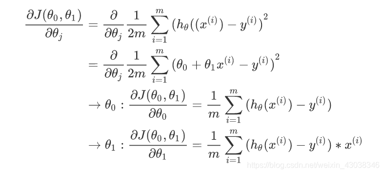
So we have gradient descent algorithm
repeat until convergence{
θ 0 : = θ 0 − α 1 m ∑ i = 1 m ( h θ ( x ( i ) ) − y ( i ) ) \theta_0 := \theta_0-\alpha\frac{1}{m} \sum_{i=1}^m{(h_{\theta}(x^{(i)})-y^{(i)})} θ0:=θ0−αm1∑i=1m(hθ(x(i))−y(i))
θ 1 : = θ 1 − α 1 m ∑ i = 1 m ( h θ ( x ( i ) ) − y ( i ) ) ∗ x ( i ) \theta_1 := \theta_1-\alpha\frac{1}{m} \sum_{i=1}^m{(h_{\theta}(x^{(i)})-y^{(i)})*x^{(i)}} θ1:=θ1−αm1∑i=1m(hθ(x(i))−y(i))∗x(i)
}
We always have a bowl shaped plot in using linear regerssion, technically is convex function(凸函数). So, instead of having many local optimum, it only has one global optimum.
“Batch” Gradient Descent
“Batch”: Each step of gradient descent uses all the training examples.
Now we have finished the first two chapter of Machine Learning, you can click here for an vivid instance produced by me in Python.
Click here to see next chapter.


 1748
1748

 被折叠的 条评论
为什么被折叠?
被折叠的 条评论
为什么被折叠?
 到【灌水乐园】发言


