神经网络（机器学习八）

前言

上一章我们结合手写数字识别的小程序学习了逻辑回归算法解决多分类问题的一般思路。这一章我们学习的是一个更加强大的分类算法：神经网络。

算法介绍

这一章，我们继续使用上一章的手写数字识别的例子，只不过，我们改成神经网络的算法。对人工智能感兴趣的同学想必都对神经网络算法不陌生，多层神经玩网络算法又叫做深度学习算法，更是大名鼎鼎了。
为什么要引入神经网络算法呢，个人理解，对于n个特征和K个待识别目标的问题，假设所有的边界都是特征的线性函数，即${\theta }^T\mathbf{x}={\theta }_0+{\theta }_1{x}_1+{\theta }_2{x}_2+\cdots +{\theta }_n{x}_n$，我们需要$n\ast K$的参数。对于更复杂一些的问题，边界不是特征的线性函数的情况，假设边界是特征的D次函数，即${\theta }^T\mathbf{x}={\theta }_0+{\theta }_1{x}_1+{\theta }_2{x}_2+\cdots +{\theta }_n{x}_n+{\theta }_{n+1}{x}_1^2+{\theta }_{n+2}{x}_2^2+\cdots +{\theta }_M{x}_n^D$，那么一共需要$O(n^D)$个参数，对于特征较多的问题，例如手写数字识别，参数的数量会随着问题的复杂程度而急剧增加，而神经网络算法可以避免出现这种情况。
　　神经网络算法采用函数嵌套的方式，既解决了非线性边界的问题，又不会引入过多的未知参数。具体来讲，一个典型的神经网络结构如下图所示，由输入层，隐藏层和输出层组成，其中输入层就是我们所选择的所有特征，输出层就是我们要识别的标签种类，而中间层呢由于大部分情况下我们也不知道代表的啥，也就是说中间这些层的信息对我们是隐藏的，所以叫就它们隐藏层了。
　　　　
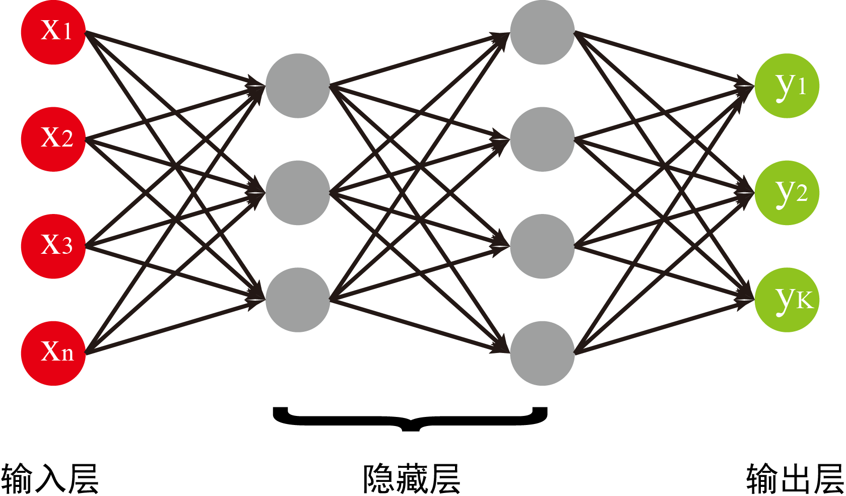
　　神经网络的工作方式就是从最左边的输入层，按照箭头的指向，向右逐层计算，最终得到输出结果。网络中的每一个箭头都代表着不同的比重参数，神经网络算法的最终目的就是找到最优的比重参数。

符号定义

为了便于表述，我们先定义一些符合来代表神经网络的一些属性。我们用大写的$L$代表神经网络的总层数，对于上图，我们有$L=4$；相应地我们用小写的$l$代表具体的某一层，$l=1,2,\cdots ,L$；按照以前的惯例，我们仍然用$n$表示特征数，用大写的$K$代表输出层的单元数，另外，我们用$S_l$代表第$l$层的单元数。
　　我们用$a_i^{(l)}$代表第$l$层的第$i$个单元，相应地，我们用没有下标的${\mathbf{a}}^{(l)}$代表第$l$层所有单元值组成的向量，显然有${\mathbf{a}}^{(1)}=\mathbf{x}$，${\mathbf{a}}^{(L)}=h_{\mathbf{\Theta }}(\mathbf{x})$。
　　我们用${\Theta }_{ji}^{(l)}$代表连接第$l$层的第$i$个单元和第$l+1$层的第$j$个单元的箭头对应的参数；相应地${\mathbf{\Theta }}^{(l)}$就表示连接第$l$层和第$l+1$层的参数矩阵，$\mathbf{\Theta }$表示所有参数组成的张量。

正向传播算法

从神经网络的输入层，逐层计算得到输出层的算法叫做正向传播（Forward Propagation）算法，具体内容如下所示：
　　　　$\begin{array}{c}{\mathbf{a}}^{(1)}=\mathbf{x}\\ {\mathbf{a}}^{(2)}=[1;g({\mathbf{\Theta }}^{(1)}{\mathbf{a}}^{(1)})]\\ {\mathbf{a}}^{(3)}=[1;g({\mathbf{\Theta }}^{(2)}{\mathbf{a}}^{(2)})]\\ ⋮\\ {\mathbf{a}}^{(L)}=[1;g({\mathbf{\Theta }}^{(L-1)}{\mathbf{a}}^{(L-1)})]\\ h_{\mathbf{\Theta }}(\mathbf{x})={\mathbf{a}}^{(L)}\end{array}$
　　其中函数$g(z)=\frac{1}{1+e^{-z}}$，$[1;g(\mathbf{\Theta }\mathbf{a})]$表示给向量$g(\mathbf{\Theta }\mathbf{a})$增加一个常数的偏置项1。可以看出隐藏层和输出层的每一个单元与上一层所有单元之间的函数关系就是逻辑回归的假设函数。通过层与层之间的嵌套，可以实现非线性边界的拟合，而神经网络中涉及的参数数目为$\sum _{l=1}^{L-1}{S}_{l+1}(S_l+1)$，远小于非线性逻辑回归算法所需的参数。

代价函数

按照以前的思路，我们需要先定义一个代价函数来指引参数优化的方向。与逻辑回归问题类似，对于神经网络，人们定义的代价函数为：
$J(\mathbf{\Theta })=-\frac{1}{m}\sum _{i=1}^m\sum _{k=1}^K[y_k^{(i)}log{h}_{\mathbf{\Theta }}({\mathbf{x}}^{(i)}{)}_k+(1-y_k^{(i)})log(1-h_{\mathbf{\Theta }}({\mathbf{x}}^{(i)}{)}_k)]+\frac{\lambda }{2m}\sum _{l=1}^{L-1}\sum _{i=1}^{S_l}\sum _{j=1}^{S_{l+1}}({\Theta }_{ji}^{(l)}{)}^2$
式中，第一项求和代表的是对所有样本的所有标签求和第二项求和是对整个$\mathbf{\Theta }$矩阵中所有元素的平方求和。

反向传播算法

接下来，与线性回归、逻辑回归等算法的思路一样，为了应用梯度下降算法，我们需要求出代价函数对每一个参数的偏导数：$\partial J/\partial \mathbf{\Theta }$。仔细观察正向传播算法就可以看出，神经网络相邻两层之间的关系就是逻辑回归中的假设函数的关系，而最终输出层与输入层之间的关系就是几层函数嵌套而成。因此要求解代价函数相对每一个参数的偏导数就需要运用链式法则，求解的结果就是反向传播算法，具体内容如下：
　　定义输出层的偏差${\delta }^{(L)}=h_{\mathbf{\Theta }}(\mathbf{x})-\mathbf{y}$；隐藏层的输出偏差可以由输出层推导出来：${\delta }^{(l)}=({\mathbf{\Theta }}^{(l)}{)}^T{\delta }^{(l+1)}.\ast {\mathbf{a}}^{(l)}.\ast (1-{\mathbf{a}}^{(l)})$，$l=2,3,\cdots ,L-1$，式中$.\ast$是Matlab中的写法，意思是矩阵中对应元素分别相乘；根据输出的偏差值，就可以计算出参数矩阵的偏导数${\mathbf{\Delta }}^{(l-1)}=({\delta }^{(l)}{)}^T{\mathbf{a}}^{(l-1)}$，$l=2,3,\cdots ,L$；再加入参数正则化项，就有：${\mathbf{D}}^{(l-1)}=\frac{1}{m}{\mathbf{\Delta }}^{(l-1)}+{\lambda }^{\ast }{\mathbf{\Theta }}^{(l-1)}$，其中${\lambda }^{\ast }=\{\begin{array}{cc}\lambda ,& >0\\ 0,& j=0\end{array}$。$\mathbf{D}$就是代价函数关于参数$\mathbf{\Theta }$的偏导数：$\frac{\partial J}{\partial {\Theta }_{ji}^{(l)}}=D_{ji}^{(l)}$。
　　这里需要注意的是偏置项的处理，由于偏置项是没有误差项的，而与偏置项相连的参数是存在偏导数的，因此，在计算${\delta }^{(l)}=({\mathbf{\Theta }}^{(l)}{)}^T{\delta }^{(l+1)}.\ast {\mathbf{a}}^{(l)}.\ast (1-{\mathbf{a}}^{(l)})$时要把$({\mathbf{\Theta }}^{(l)}{)}^T{\delta }^{(l+1)}$中与偏置项对应的那个数去掉。
　　至此，我们就完成了梯度下降算法所需的所有计算，接下来的任务就是运行梯度下降算法，寻找最优的参数了。

算法实现

利用神经网络算法实现手写数字识别的MataLab程序如下所示。程序中使用单元数依次为400,30,30,10的神经网络，初始值为0到0.1之间的随机数，$\lambda =0.0005$，得到的准确率约为$93.6\%$，比上一章使用的非线性逻辑回归算法更高一些。
　　这里需要注意的是，对于$\mathbf{\Theta }$和$\lambda$的初始化。$\mathbf{\Theta }$的初始值不能像之前一样全部设为0，而是采用随机数进行初始化。另外，初始的$\mathbf{\Theta }$和$\lambda$不能太大，否则梯度下降算法也难以在有限的步数内优化到最小值。

clear all;
close all;
clc;

load('ex3\ex3data1.mat');
load('ex3\ex3weights.mat');

X0=X;
y0=y;

M=size(X,1);
%Get the tranning set.
m=round(M*0.7);
rand_indices=randperm(M);
X=X(rand_indices(1:m),:);
y=y(rand_indices(1:m),:);

%Get the labels of the trainning set.
Y=zeros(m,10);
for i=1:m
    Y(i,y(i))=1;
end

%nnet defines number of units in each layer.
nnet=[400;30;30;10];

%Calculate the total number of parameters.
n=0;
for i=1:length(nnet)-1
    n=n+(nnet(i)+1)*nnet(i+1);
end

%Initiate the parameter theta and lambda.
theta=rand(n,1)*0.1;
lamda=5e-4;

%Calculate the cost,gradient,and hypothesis value of the neural net.
[J,grad,h]=CostFuncNeu(theta,nnet,X,Y,lamda);

%Check the validity of CostFuncNeu by comparing it with neumeric method,
%which should be ignored when formally running the program.
%%Gradient checking...
% grad1=grad;
% for i=n-100:n
%     theta(i)=theta(i)+0.00001;
%     [cost1,g]=CostFuncNeu(theta,nnet,X,Y,lamda);
%     theta(i)=theta(i)-0.00002;
%     [cost2,g]=CostFuncNeu(theta,nnet,X,Y,lamda);
%     theta(i)=theta(i)+0.00001;
%     grad1(i)=(cost1-cost2)/0.00002;
%     i
% end
% check=[grad,grad1]
%%Gradient checking end.

%Optimize the parameter theta through gradient descent method.
%OptimizationMethod1
options=optimset('GradObj', 'on', 'MaxIter', 500);
[theta,cost]=fmincg(@(t)(CostFuncNeu(t,nnet,X,Y,lamda)),theta,options);

%OptimazationMethod2
% alpha=10;
% for step=1:500
%     [cost,grad,h]=CostFuncNeu(theta,nnet,X,Y,lamda);
%     theta=theta-alpha*grad;
%     alpha=alpha*1.001;
%     cost
% end


%Get the test set. 
X=X0(rand_indices(m+1:end),:);
y=y0(rand_indices(m+1:end),:);

%Get the prediction result.
Y=zeros(length(y),10);
for i=1:length(y)
    Y(i,y(i))=1;
end
[cost,grad,h]=CostFuncNeu(theta,nnet,X,Y,lamda);
result=[y,h];
[value,index]=max(h,[],2);
 
 %Check the accuracy of prediction.
accuracy=sum(index==y)/length(y);



%Display the predicting process
figure,
for i=1:300
    data=X(i,:);
    img=reshape(data,20,20);
    %subplot(10,10,i),
    img=imresize(img,30);
    imshow(img);
    
    [p,o,h]=CostFuncNeu(theta,nnet,X(i,:),Y(i,:),lamda);
    
    [value,index]=max(h);
    if index==10
        index=0;
    end 
    label=y(i);
    if label==10
        label=0;
    end
    xlabel([num2str(label),',',num2str(index),'(',num2str(value),')']);
    drawnow;
    pause(1.5);   
end

function [J,grad,h]=CostFuncNeu(theta,nnet,X,y,lamda)
%m is the quantity of sample.
m=length(X(:,1));
%nnet is organized like this:
%[units of layer1(input layer); units of layer2;...,units of layer
%L(output)],No bias unit counted.
L=length(nnet);
index=1;
Theta=cell(L-1,1);
Lamda=cell(L-1,1);
for i=1:L-1
    Theta{i}=reshape(theta(index:index+nnet(i+1)*(nnet(i)+1)-1),nnet(i+1),(nnet(i)+1));
    index=index+nnet(i+1)*(nnet(i)+1);
    Lamda{i}=ones(nnet(i+1),(nnet(i)+1))*lamda;
    Lamda{i}(:,1)=0;
end

%Forward calculation of the hypothesis values.
a=cell(L,1);
z=cell(L,1);
a{1}=[ones(m,1),X];
z{1}=0;
for i=2:L
    z{i}=a{i-1}*Theta{i-1}';
    if i==L
        a{i}=Sigmoid(z{i});
    else
        a{i}=[ones(m,1),Sigmoid(z{i})];
    end
end
h=a{L};

%Backward propagation.
delta=cell(L,1);
Delta=cell(L-1,1);
D=cell(L-1,1);
delta{L}=h-y;
for i=L-1:-1:2
    if i==L-1
        delta{i}=delta{i+1}*Theta{i}.*a{i}.*(1-a{i});
    else
        delta{i}=delta{i+1}(:,2:end)*Theta{i}.*a{i}.*(1-a{i});
    end
end


for i=L-1:-1:1
    if i==L-1
        Delta{i}=delta{i+1}'*a{i};
    else
        Delta{i}=delta{i+1}(:,2:end)'*a{i};
    end
    D{i}=1/m*Delta{i}+2*Lamda{i}.*Theta{i};
end

%Reshape the gradient to size of theta
grad=zeros(size(theta));
index=1;
for i=1:L-1
    [a,b]=size(D{i});
    grad(index:index+a*b-1)=reshape(D{i},a*b,1);
    index=index+a*b;
end

cost=-1/m*(y.*log(h)+(1-y).*log(1-h));
J=sum(cost(:));
for i=1:L-1
    cost=Lamda{i}.*Theta{i}.^2;
    J=J+sum(cost(:));
end