


 本文介绍了MATLAB中的histogram和histogram2函数,用于绘制直方图。histogram函数详细讲解了计数功能、频率分布、指定边界以及属性设置。histogram2函数则用于绘制二维直方图。文章还提到了morebins、fewerbins、histcounts和histcounts2等辅助函数,它们用于调整条目数量和统计计数。

MATLAB中所有的线图已经讲完了,从本文开始,将花几篇文章陆续讲述MATLAB的数据分布图。
数据分布图包含三种类型图,即
- 直方图和箱线图。包括:histogram、histogram2、morebins、fewerbins、histcounts、histcounts2、boxchart函数;
- 散点图和平行坐标。包括:scatter、scatter3、binscatter、scatterhistogram、spy、plotmatrix、parallelplot函数;
- 饼图、热图和文字云。包括:pie、pie3、heatmap、sortx、sorty、wordcloud函数。
在科研遇到统计数据时,这几类图用得非常广泛,在顶刊Nature和Science中经常看到。毕竟,好的统计结果以及好的可视化能让文章质量增加很多。
本文将从直方图开始,讲述histogram和histogram2函数的用法和示例。morebins、fewerbins、histcounts、histcounts2这几个函数并没有画图功能,而是histogram函数的辅助,用于设定或者求解某些值,也将在本文一并讲解。
注意、注意、注意,histogram用的非常多,具备数据分组和画图功能,非常强大。科研非常常见,用法也比较复杂,此文内容较为重要。
另外,需要区别histogram函数和bar函数。histogram函数是直方图,注重于统计,而bar是条形图,在图形方面设置更多。某些情况,两者可以一致。
1 histogram函数
1.1 用法
histogram(X)
histogram(X,nbins)
histogram(X,edges)
histogram('BinEdges',edges,'BinCounts',counts)
histogram(C)
histogram(C,Categories)
histogram('Categories',Categories,'BinCounts',counts)
histogram(___,Name,Value)
histogram(ax,___)
h = histogram(___)
histogram(X) 基于 X 创建直方图。histogram 函数使用自动 bin 划分算法,然后返回均匀宽度的 bin,这些 bin 可涵盖 X 中的元素范围并显示分布的基本形状。histogram 将 bin 显示为矩形,这样每个矩形的高度就表示 bin 中的元素数量。例如,histogram(X,nbins) 使用标量 nbins 指定的 bin 数量。histogram(X,edges) 将 X 划分到由向量 edges 来指定 bin 边界的 bin 内。每个 bin 都包含左边界,但不包含右边界,除了同时包含两个边界的最后一个 bin 外。
histogram('BinEdges',edges,'BinCounts',counts) 手动指定 bin 边界和关联的 bin 计数。histogram 绘制指定的 bin 计数,而不执行任何数据的 bin 划分。例如,histogram(C)(其中 C 为分类数组)通过为 C 中的每个类别绘制一个条形来绘制直方图。
histogram(C,Categories) 仅绘制 Categories 指定的类别的子集。
histogram('Categories',Categories,'BinCounts',counts) 手动指定类别和关联的 bin 计数。histogram 绘制指定的 bin 计数,而不执行任何数据的 bin 划分。例如,histogram(___,Name,Value) 使用前面的任何语法指定具有一个或多个 Name,Value 对组参数的其他选项。例如,可以指定 'BinWidth' 和一个标量以调整 bin 的宽度,或指定 'Normalization' 和一个有效选项('count'、 'probability'、 'countdensity'、 'pdf'、 'cumcount' 或 'cdf' )以使用不同类型的归一化。有关属性列表,请参阅 Histogram 属性。
histogram(ax,___) 将图形绘制到 ax 指定的坐标区中,而不是当前坐标区 (gca) 中。选项 ax 可以位于前面的语法中的任何输入参数组合之前。例如,h = histogram(___) 返回 Histogram 对象。使用此语法可检查并调整直方图的属性。有关属性列表,请参阅 Histogram 属性。[1]
接下来请看具体示例。
1.2 示例1
clc
clear all
close all
a = randn(10000,1);
subplot(1,2,1)
h1 = histogram(a);
subplot(1,2,2)
h2 = histogram(a,20);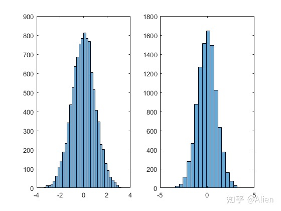
首先我们生成均值为0,标准差为1的正太分布,上图为统计结果。直方图有很多属性,可在赋值h中查看,可以直接对属性进行更改。
例如,作图为默认,通过
n1 = h1.NumBins我们可以查询条的个数为41。在画图时,可以更改属性,例如设置为20个条
h2 = histogram(a,20);如上右图所示。
1.3 计数功能和频率
请注意,这一小节非常、非常有用!!!
histogram函数可以通过属性,查询每个条的边界坐标、个数和宽度,这样我们可以计算频率。Ps: histogram可以自行绘制PDF,但这里我们手动计算和绘制。
边界坐标、数量和宽度分别可以通过下面属性进行
BinCounts
BinEdges
BinWidth
求频率分布如下
clc
clear all
close all
a = randn(10000,1);

figure(1)
subplot(1,2,1)
h1 = histogram(a);
L = length(h1.BinEdges);
for i = 1:L-1
    x1(i) = (h1.BinEdges(i) + h1.BinEdges(i+1))/2;
end
y1 = h1.Values/10000/h1.BinWidth;
figure(2)
plot(x1,y1,'s','linewidth',2,'MarkerSize',10)

figure(1)
subplot(1,2,2)
h2 = histogram(a,20);
L = length(h2.BinEdges);
for i = 1:L-1
    x2(i) = (h2.BinEdges(i) + h2.BinEdges(i+1))/2;
end
y2 = h2.Values/10000/h2.BinWidth;
figure(2)
hold on
plot(x2,y2,'o','linewidth',2,'MarkerSize',10)
xlim([-4,4])
首先,通过
(h1.BinEdges(i)+ h1.BinEdges(i+1))/2求每个条中点的坐标。由于每个小条的面积就是频率,可通过
h1.Values/h1.BinWidth/10000求每个条的高度。频率图如下
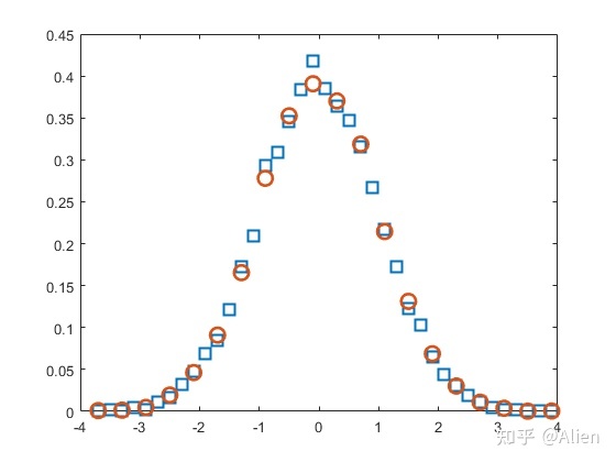
在1.2节中,不同分类条的高度是不同的,在这里,是一致的。
当然,上面是原理,下面利用MATLAB的属性来绘制。
MATLAB中可以直接将图的属性设置为'PDF',即频率分布,如
histogram(x,'Normalization','pdf')下面是示例。
clc
clear all
close all
a = randn(10000,1);
h1 = histogram(a,21,'Normalization','pdf');
hold on
x = -4:0.1:4;
mu = 0;
sigma = 1;
y = exp(-(x-mu).^2./(2*sigma^2))./(sigma*sqrt(2*pi));
plot(x,y,'LineWidth',1.5)
figure(2)
h2 = histogram(a,21);
L = length(h2.BinEdges);
for i = 1:L-1
    x2(i) = (h2.BinEdges(i) + h2.BinEdges(i+1))/2;
end
y2 = h2.Values/10000/h2.BinWidth;
figure(1)
hold on
plot(x2,y2,'o','linewidth',1.5,'MarkerSize',8)
xlim([-4,4])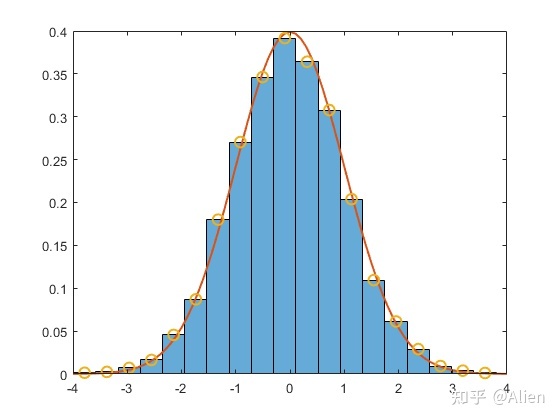
点是我们自己计算的,可以发现计算结果与MATLAB一致,另外,标准正态分布概率密度函数为

令
 带入,画在图中,可以看出频率与概率吻合较好。
除了pdf(频率),还有
- 'count':计数,默认格式,
 ,为观测值的计数或频率;
 - 'countdensity':
 ,按条的宽度进行换算的计数或频率。
 - 'cumcount':
 ,累积计数。每个条的值等于该条及以前的所有条中的累积观测值数量。
 - 'probability':
 ,相对概率。
 - 'pdf':
 ,概率密度函数的估计值。
 - 'cdf':
 ,累积的密度函数估算值。
1.4 指定边界
在上面画图时,边界是默认的。histogram函数一般查找一组数据最大值和最小值,然后再分组。然而,当数据有一数据非常偏离时(实验中非常常见),会影响可视化效果,例如我在数据中添加了一个数据值15,图形如下所示。
原本是分类为20组,但是这个数据影响了分类,比较直观结果只有7组,其他的为0。
clc
clear all
close all
a = randn(10000,1);
a(10001,1) = 15;
h1 = histogram(a,20);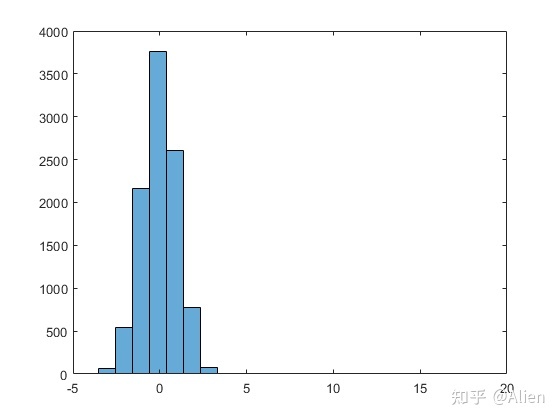
但histogram函数中,我们可以指定边界,并指定宽度,例如这里边界为-20到-4以及4到20,分别只产生一个条,-4到4每隔0.4产生一个条,即一共生成1+20+1=22个条。
clc
clear all
close all
a = randn(10000,1);
a(10001,1) = 15;
edges = [-20 -4:0.4:4 20];
subplot(1,2,1)
h1 = histogram(a,edges);
subplot(1,2,2)
h2 = histogram(a,edges);
xlim([-4,4])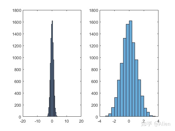
这样可以将偏离值抽象掉,如左图所示。并通过调整x轴范围,得到可视化效果较好的图,如右图所示。
此方法处理实验数据时,非常常见,有的人可能通过删除点的方式来实现,而我不建议这么做。
另外,建议当数据是对称时,条的个数最好设置为奇数。
1.5 求他属性
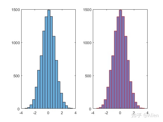
其他属性主要是设定每个条的边界颜色和面颜色。示例如下
clc
clear all
close all
a = randn(10000,1);
subplot(1,2,1)
h1 = histogram(a,21);
xlim([-4,4])
subplot(1,2,2)
h2 = histogram(a,21);
h2.FaceColor = [0.1 0.1 0.5];
h2.EdgeColor = 'r';
xlim([-4,4])
这里通过FaceColor更改面颜色,通过EdgeColor更改边颜色。
1.6 绘制多个直方图
MATLAB可以将多个直方图绘制在一起,便于进行对比,例如
clc
clear all
close all
a = randn(10000,1)-2;
h1 = histogram(a,21);
b = randn(10000,1);
hold on
h2 = histogram(b,21);
c = randn(10000,1)+2;
hold on
h3 = histogram(c,21);
xlim([-6,6])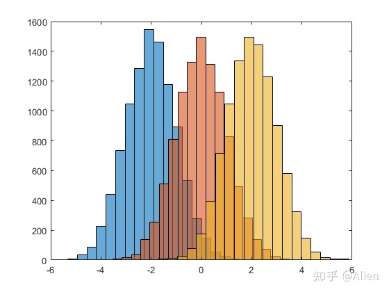
当然,histogram还有一些其他小功能,这里不赘述了,可以在属性中进行查找,或者参阅帮助文档[1]。
2 histogram2函数
histogram2函数即二维直方图。用法和histogram函数基本一致,但略有区别。
2.1 示例1
clc
clear all
close all
a = randn(50000,1);
b = randn(50000,1);
subplot(2,2,1)
h1 = histogram2(a,b);
xlim([-4,4])
ylim([-4,4])
subplot(2,2,2)
h2 = histogram2(a,b,20);
xlim([-4,4])
ylim([-4,4])
subplot(2,2,3)
h3 = histogram2(a,b);
axis([-4,4,-4,4])
subplot(2,2,4)
h4 = histogram2(a,b,20);
axis([-4,4,-4,4])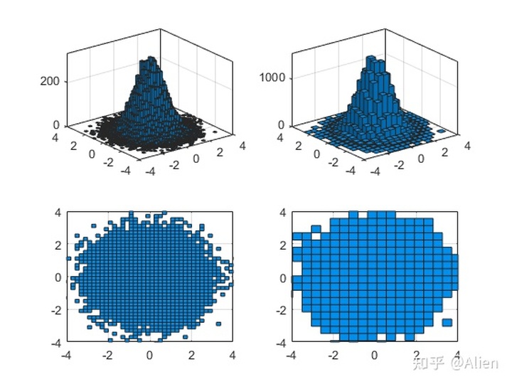
左边是默认分组,并有两个视角;右边是x和y方向都分成20组,并有两个视角,和histogram函数基本一致。
采用句柄 h.NumBins可查询分组数目,采用h.Values可以看分组情况。
如果要x和y分组不一样,采用
histogram2(a,b,[m,n]);例如
clc
clear all
close all
a = randn(50000,1);
b = randn(50000,1);
subplot(2,2,1)
h1 = histogram2(a,b,[15,5]);
xlim([-4,4])
ylim([-4,4])
subplot(2,2,2)
h2 = histogram2(a,b,[5,15]);
xlim([-4,4])
ylim([-4,4])
subplot(2,2,3)
h3 = histogram2(a,b,[15,5]);
axis([-4,4,-4,4])
subplot(2,2,4)
h4 = histogram2(a,b,[5,15]);
axis([-4,4,-4,4])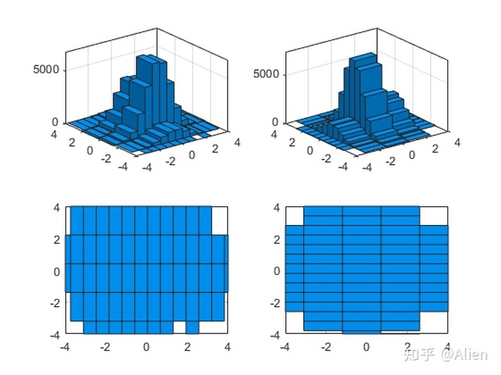
左图将x分成15组,y分成5组;右图将x分成5组,y分成15组。
2.2 示例2
histogram2函数可以对高度进行着色,色彩根据高度而定,例如
clc
clear all
close all
a = randn(50000,1);
b = randn(50000,1);
subplot(2,2,1)
h1 = histogram2(a,b,[10,10],'FaceColor','flat');
xlim([-4,4])
ylim([-4,4])
subplot(2,2,2)
h2 = histogram2(a,b,[25,25],'FaceColor','flat');
xlim([-4,4])
ylim([-4,4])
subplot(2,2,3)
h3 = histogram2(a,b,[10,10],'FaceColor','flat');
axis([-4,4,-4,4])
subplot(2,2,4)
h4 = histogram2(a,b,[25,25],'FaceColor','flat');
axis([-4,4,-4,4])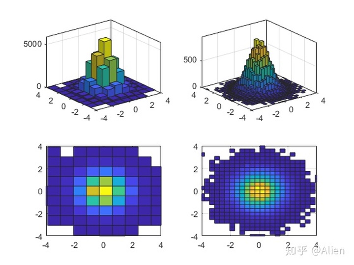
其余用法和histogram函数一致,例如指定边界、设定为频率分布图等等,这里不再赘述。
3 其余函数
其余函数主要包括morebins、fewerbins、histcounts、histcounts2这几个函数,他们并没有画图功能,主要配合histogram函数使用。
3.1 morebins和fewerbins函数
morebins和fewerbins函数主要用于稍微精细调整条的数目,morebins函数增加,fewerbins函数减少。
例如
clc
clear all
close all
a = randn(10000,1);
h1 = histogram(a);
h1.NumBins
morebins(h1)
h2 = histogram(a);
h2.NumBins
fewerbins(h2)
默认分组为39,morebins函数使分组数目增加至43,fewerbins函数减少至35。
3.2 histcounts和histcounts2函数
此函数主要对直方图的条数进行分组和计数,与histogram和histogram2函数相比,功能一致,但不能画图。
例如
[N,edges] = histcounts(X)返回分组数目和边界;
[N,edges] = histcounts(X,nbins)指定分组数目;
edges = [-5:0.2:1];
N = histcounts(X,edges)
指定边界;
[N,edges] = histcounts(X, 'Normalization', 'probability')指定数据类型等等,例如PDF。
histcounts2函数一致,这里不再赘述,参考[2][3]。
持续更新,更多文章请见目录
MATLAB画图技巧与实例:目录
Alien:MATLAB画图技巧与实例:目录zhuanlan.zhihu.com
MATLAB画图技巧与实例(一):常用函数
Alien:MATLAB画图技巧与实例(一):常用函数zhuanlan.zhihu.com
参考
- ^abMATLAB帮助文档 https://ww2.mathworks.cn/help/matlab/ref/matlab.graphics.chart.primitive.histogram.html
- ^https://ww2.mathworks.cn/help/matlab/ref/matlab.graphics.chart.primitive.histogram2.html
- ^https://ww2.mathworks.cn/help/matlab/pie-charts-bar-plots-and-histograms.html?s_tid=CRUX_lftnav


 被折叠的 条评论
为什么被折叠?
被折叠的 条评论
为什么被折叠?
 到【灌水乐园】发言


