


项目描述:数据里涵盖从2010年12月1号到2011年12月9号期间在英国注册的在线零售店发生的所有在线交易,希望从中挖掘出有用的信息,特别是用户层面
项目数据来源:kaggle
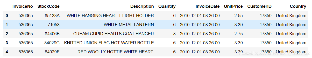
数据字段:
- InvoiceNo: 发票编号。6位整数。如果代码以字母“c”开头,则表示是一个退货订单
- StockCode: 商品代码。为每个不同的产品唯一分配的5位整数
- Description: 商品描述
- Quantity:商品数量
- InvoiceDate:发票日期
- UnitPrice:单价。英镑单位的产品价格
- CustomerID:客户编码
- Country:每个客户所在的国家
模块导入和数据导入
import pandas as pd
import datetime
import math
import numpy as np
import matplotlib.pyplot as plt
import matplotlib.mlab as mlab
import matplotlib.cm as cm

%matplotlib inline

import seaborn as sns
sns.set(style="ticks", color_codes=True, font_scale=1.5)
color = sns.color_palette()
sns.set_style('darkgrid')

from scipy import stats
from scipy.stats import skew, norm, probplot, boxcox
from sklearn import preprocessing

from sklearn.cluster import KMeans
from sklearn.metrics import silhouette_samples, silhouette_score
#from IPython.display import display, HTML

from mpl_toolkits.mplot3d import Axes3D

import plotly as py
import plotly.graph_objs as go
py.offline.init_notebook_mode()
import datetime as dt
from IPython.core.interactiveshell import InteractiveShell
InteractiveShell.ast_node_interactivity = "all"
# IDs are not numerical but strings
df_initial = pd.read_excel("Online Retail.xlsx",dtype={'CustomerID': str,'InvoiceNo': str})
Data Munipulation
df_M = df_initial
df_M.head(5)
#删除重复值
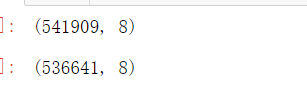
df_M.shape
df_M.drop_duplicates(inplace= True)
df_M.shape
# 时间列调整
df_M['InvoiceDate'] = pd.to_datetime(df_M['InvoiceDate'])
df_M['Date'] = pd.to_datetime(df_M['InvoiceDate'].dt.date, errors='coerce')
df_M.describe()
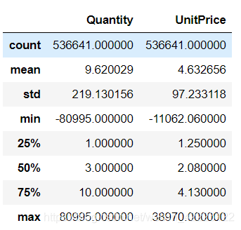
发现有负值,应该是退款单的
# 检查类型和是否有空值
df_M.info()
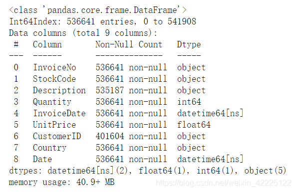
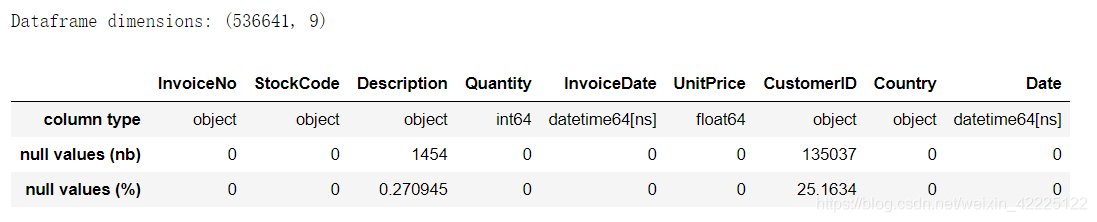
我们发现Description和CustomerID有明显的缺失
# 数据处理
print('Dataframe dimensions:', df_M.shape)
# gives some infos on columns types and numer of null values
tab_info=pd.DataFrame(df_M.dtypes).T.rename(index={0:'column type'})
tab_info=tab_info.append(pd.DataFrame(df_M.isnull().sum()).T.rename(index={0:'null values (nb)'}))
tab_info=tab_info.append(pd.DataFrame(df_M.isnull().sum()/df_M.shape[0]*100).T.rename(index={0:'null values (%)'}))
display(tab_info)
display(df_M[:5])

# 放弃没有用户ID的
df_M = df_M[~(df_M.CustomerID.isnull())]

# 放弃单价为0的
df_M = df_M[df_M.UnitPrice!=0]
df_M.isnull().sum()
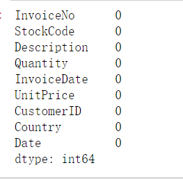
print('去除了百分之',round((541909-df_M.shape[0])/541909*100,2))
去除了百分之 25.9
# 重新规整数字类型
df_M['Quantity'] = df_M['Quantity'].astype('int32')
df_M['UnitPrice'] = df_M['UnitPrice'].astype('float')
df_M['CustomerID'] = df_M['CustomerID'].astype('int32')
df_M['InvoiceNo'] = df_M['InvoiceNo'].astype('str')
# 增加消费金额这列
df_M['SumPrice']=df_M['UnitPrice']*df_M['Quantity']
客户消费行为分析
客户生命周期
# 建立副本
df=df_M.copy()
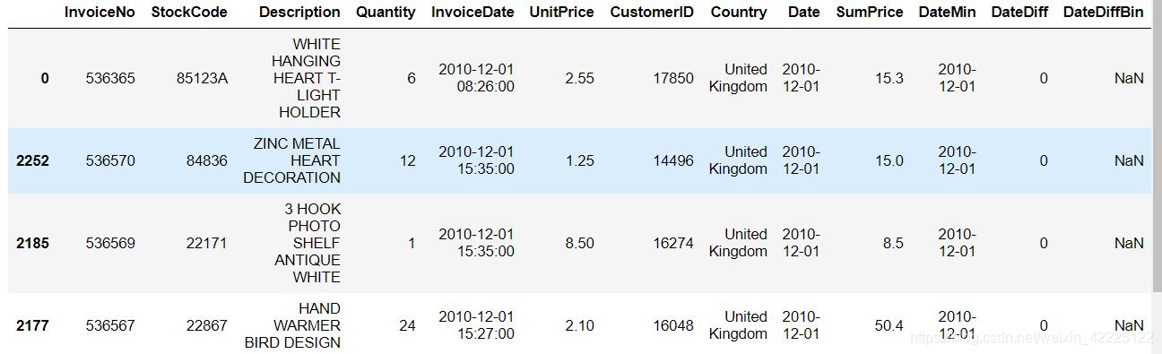
df.head()
查看用户的初次与末次(最近)消费时间:
# 客户的初次消费时间
mindate = df.groupby('CustomerID')[['Date']].min()
# 客户的末次消费时间
maxdate = df.groupby('CustomerID')[['Date']].max()
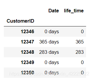
# 客户的消费周期
life_time=(maxdate - mindate)
life_time.head()
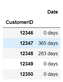
# 转换为数值
life_time['life_time'] = life_time['Date'].dt.days
# 客户周期分布
fig=plt.figure(figsize=(12,6))
sns.distplot(life_time[life_time['life_time']>0].life_time,bins=30,color='g')
plt.title('Life Time Distribution')
plt.ylabel('Customer number')
plt.xlabel('Life time (days)')
plt.show()
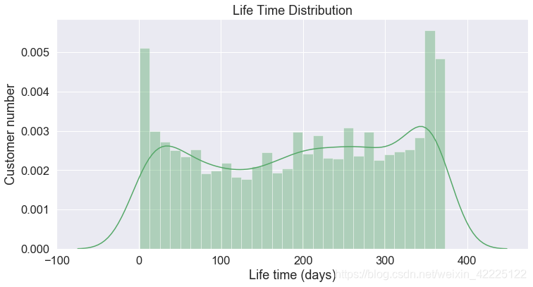
- 大部分客户的消费周期还是偏向于短期
- 由于选取数据周期的原因,客户的生命周期有可能还在往后延伸
# 平均用户周期为
life_time[life_time['life_time'] > 0].life_time.mean()
life_time.life_time.mean()
195.4653961885657
133.75360329444064
说明客户消费一次后再次引导消费的成功率应该会提高
用户留存分析
假设在这段周期内的用户首次消费为他的初次消费
#通过内表连接df和mindate,计算顾客每次消费日期与顾客任意一次消费的差距
customer_retention = pd.merge(df, mindate, left_on='CustomerID', right_index=True, how='inner', suffixes=('', 'Min'))
customer_retention['DateDiff'] = (customer_retention.Date - customer_retention.DateMin).dt.days
date_bins = [0, 3, 7, 30, 60, 90, 180,500]
customer_retention['DateDiffBin'] = pd.cut(customer_retention.DateDiff, bins = date_bins)
customer_retention['DateDiffBin'].value_counts()
(180, 500] 141390
(90, 180] 76328
(30, 60] 29062
(60, 90] 26447
(7, 30] 18574
(3, 7] 4128
(0, 3] 1855
Name: DateDiffBin, dtype: int64
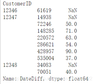
retention_pivot = customer_retention.pivot_table(index = ['CustomerID'], columns = ['DateDiffBin'], values = ['SumPrice'], aggfunc= np.sum)
print(retention_pivot)
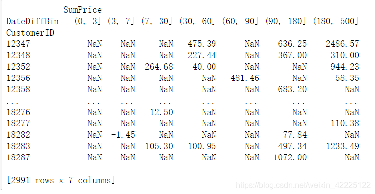
通过这个表可以计算出每个顾客在固定周期(比如3天,7天的总消费或者平均消费)
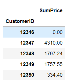
# 每位顾客的LCTV(用户生命周期价值)
df_S=df.groupby('CustomerID')['SumPrice'].sum()
df_S=pd.DataFrame(df_S)
df_S.head()
life_time.head()
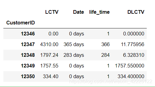
# 每位顾客的日均LCTV
df_SL = pd.merge(df_S, life_time, left_on='CustomerID', right_index=True, how='inner')
df_SL['life_time']=df_SL['life_time']+1
df_SL['DLCTV']=df_SL.SumPrice/df_SL.life_time
df_SL.rename(columns={'SumPrice':'LCTV'},inplace=True)
df_SL.head()
客户购买周期分析
# 去掉重复数据
sales_cycle = customer_retention.drop_duplicates(subset=['CustomerID', 'Date'], keep='first')
sales_cycle.sort_values(by = 'Date',ascending = True).head()
# 定义相邻差分函数
def diff(group):
    d = group.DateDiff - group.DateDiff.shift()
    return d
last_diff = sales_cycle.groupby('CustomerID').apply(diff)
last_diff.head(10)
last_diff_customer = last_diff.groupby('CustomerID').mean()
last_diff_customer.hist(bins = 50, figsize = (12, 6), color = 'c')
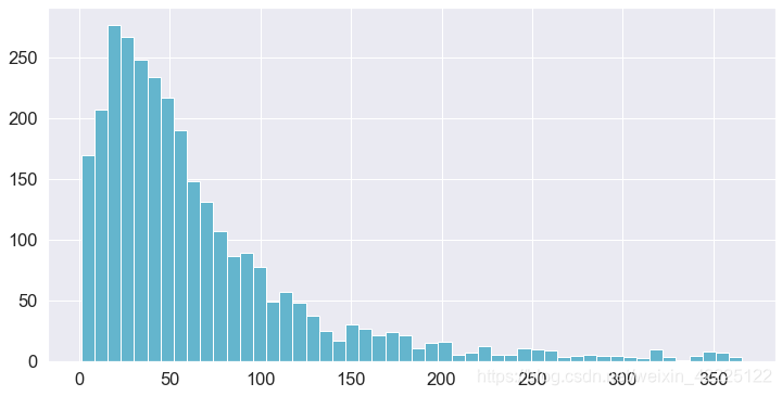
大部分的复购日期在20天左右
RFM模型
Recency
df1=df.copy()
refrence_date = df1.InvoiceDate.max() + datetime.timedelta(days = 1)
print('Reference Date:', refrence_date)
df1['days_since_last_purchase'] = (refrence_date - df1.InvoiceDate).astype('timedelta64[D]')
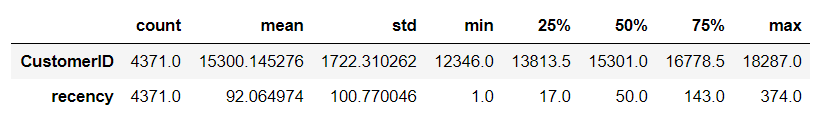
customer_history_df = df1[['CustomerID', 'days_since_last_purchase']].groupby("CustomerID").min().reset_index()
customer_history_df.rename(columns={'days_since_last_purchase':'recency'}, inplace=True)
customer_history_df.describe().transpose()
#检验是否正态分布的QQ图
def QQ_plot(data, measure):
    fig = plt.figure(figsize=(20,7))

    #Get the fitted parameters used by the function
    (mu, sigma) = norm.fit(data)

    #Kernel Density plot
    fig1 = fig.add_subplot(121)
    sns.distplot(data, fit=norm)
    fig1.set_title(measure + ' Distribution ( mu = {:.2f} and sigma = {:.2f} )'.format(mu, sigma), loc='center')
    fig1.set_xlabel(measure)
    fig1.set_ylabel('Frequency')

    #QQ plot
    fig2 = fig.add_subplot(122)
    res = probplot(data, plot=fig2)
    fig2.set_title(measure + ' Probability Plot (skewness: {:.6f} and kurtosis: {:.6f} )'.format(data.skew(), data.kurt()), loc='center')

    plt.tight_layout()
    plt.show()
QQ_plot(customer_history_df.recency, 'Recency')
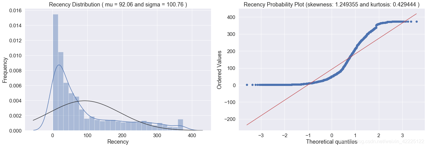
发现不是很符合,总体分布偏右偏
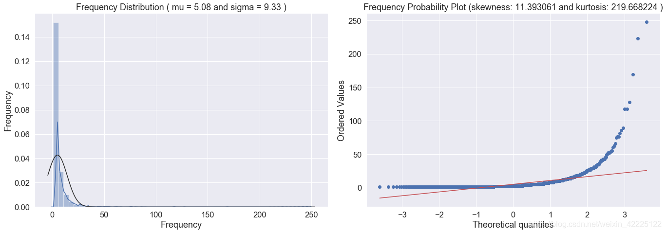
Frequency
customer_freq = (df1[['CustomerID', 'InvoiceNo']].groupby(["CustomerID", 'InvoiceNo']).count().reset_index()).\
                groupby(["CustomerID"]).count().reset_index()
customer_freq.rename(columns={'InvoiceNo':'frequency'},inplace=True)
customer_history_df = customer_history_df.merge(customer_freq)
QQ_plot(customer_history_df.frequency, 'Frequency')
Monetary Value
customer_monetary_val = df1[['CustomerID', 'SumPrice']].groupby("CustomerID").sum().reset_index()
customer_history_df = customer_history_df.merge(customer_monetary_val)
customer_history_df.rename(columns={'SumPrice':'monetary'}, inplace=True)
QQ_plot(customer_history_df.monetary, 'monetary')
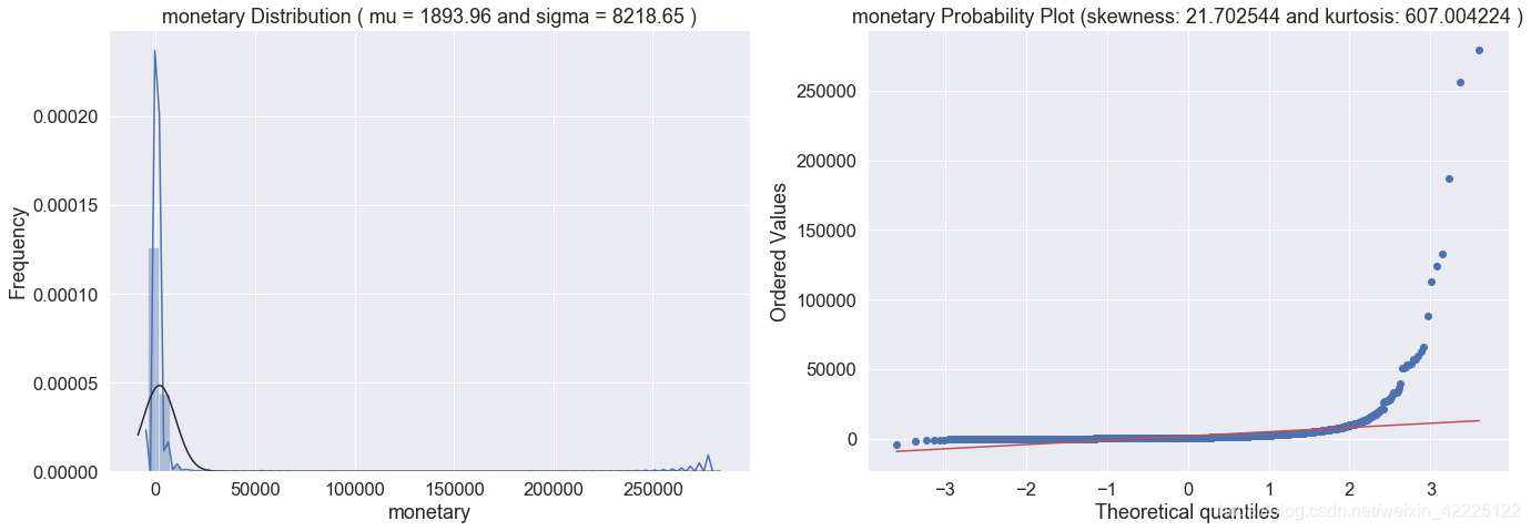
超级不符合正态分布
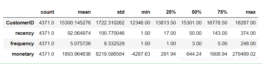
customer_history_df.describe().transpose()
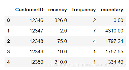
rfmTable = customer_history_df
rfmTable.head(5)
打分
# 四分位打分法
quantiles = rfmTable.quantile(q=[0.25,0.5,0.75])
quantiles = quantiles.to_dict()
segmented_rfm = rfmTable
#划分后临界点数据
quantiles
{‘CustomerID’: {0.25: 13813.5, 0.5: 15301.0, 0.75: 16778.5},
‘recency’: {0.25: 17.0, 0.5: 50.0, 0.75: 143.0},
‘frequency’: {0.25: 1.0, 0.5: 3.0, 0.75: 5.0},
‘monetary’: {0.25: 291.94, 0.5: 644.2400000000001, 0.75: 1608.94}}
# 定义划分函数
def RScore(x,p,d):
    if x <= d[p][0.25]:
        return 1
    elif x <= d[p][0.50]:
        return 2
    elif x <= d[p][0.75]:
        return 3
    else:
        return 4

def FMScore(x,p,d):
    if x <= d[p][0.25]:
        return 4
    elif x <= d[p][0.50]:
        return 3
    elif x <= d[p][0.75]:
        return 2
    else:
        return 1
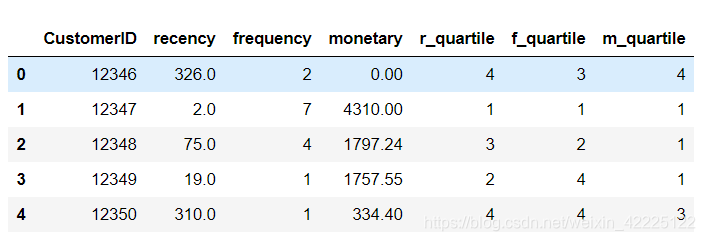
segmented_rfm['r_quartile'] = segmented_rfm['recency'].apply(RScore, args=('recency',quantiles,))
segmented_rfm['f_quartile'] = segmented_rfm['frequency'].apply(FMScore, args=('frequency',quantiles,))
segmented_rfm['m_quartile'] = segmented_rfm['monetary'].apply(FMScore, args=('monetary',quantiles,))
segmented_rfm.head(5)
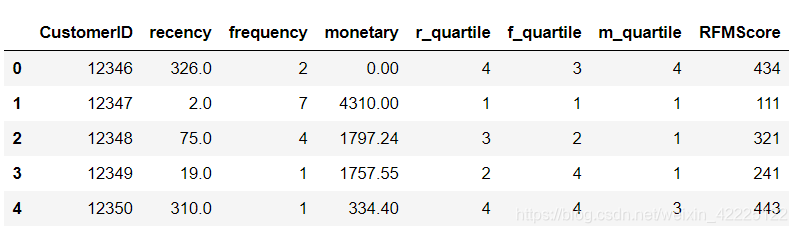
# 联合打分
segmented_rfm['RFMScore'] = segmented_rfm.r_quartile.map(str) \
                              + segmented_rfm.f_quartile.map(str) \
                              + segmented_rfm.m_quartile.map(str)

segmented_rfm.head(5)
| R分段 | 得分 | F分段 | 得分 | M分段 | 得分 |
|---|---|---|---|---|---|
| 活跃用户 | 1 | 忠实客户 | 1 | 高贡献 | 1 |
| 沉默用户 | 2 | 成熟客户 | 2 | 中高贡献 | 2 |
| 睡眠用户 | 3 | 老客户 | 3 | 中贡献 | 3 |
| 流失用户 | 4 | 新客户 | 4 | 低贡献 | 4 |
分数越低客户越有价值,最有价值客户标签为‘111’,最没有价值客户标签为‘444’
将客户分为四个不同层次后可以暂时分成四大营销方向:
- 0 - 122,:最有价值客户 方案:倾斜更多资源,VIP服务,个性化服务及附加销售等
- 122 - 223:一般价值客户 方案:提供会员、积分等计划,推荐其他相关产品
- 223 - 333: 潜在流失客户 方案:加强联系,提高留存
- 333以上: 流失客户 方案 :以促销折扣等方式恢复客户兴趣,否则暂时放弃无价值的客户
部分代码借鉴于:https://blog.youkuaiyun.com/qq_42615032/article/details/103127935


 被折叠的 条评论
为什么被折叠?
被折叠的 条评论
为什么被折叠?
 到【灌水乐园】发言


