


记录一下
embedding_lookup 词向量
根据词的索引来获取embedding
输入是[batch_size,seq_lenth] 输出[batch_size,seq_lenth,embeding_size]
def embedding_lookup(input_ids,
                     vocab_size,
                     embedding_size=128,
                     initializer_range=0.02,
                     word_embedding_name="word_embeddings",
                     use_one_hot_embeddings=False):
  """Looks up words embeddings for id tensor.

  input_ids: int32 Tensor shape为[batch_size, seq_length],表示WordPiece的id
		vocab_size: int 词典大小,需要于vocab.txt一致
		embedding_size: int embedding后向量的大小
		initializer_range: float 随机初始化的范围
		word_embedding_name: string 名字,默认是"word_embeddings"
		use_one_hot_embeddings: bool 如果True,使用one-hot方法实现embedding;否则使用
			`tf.nn.embedding_lookup()`. TPU适合用One hot方法。
  """

  # 这个函数假设输入的shape是[batch_size, seq_length, num_inputs]
  # 普通的Embeding一般假设输入是[batch_size, seq_length],
  # 增加num_inputs这一维度的目的是为了一次计算更多的Embedding
  # 但目前的代码并没有用到,传入的input_ids都是2D的,这增加了代码的阅读难度。

  # 如果输入是[batch_size, seq_length],
  # 那么我们把它 reshape成[batch_size, seq_length, 1]
  if input_ids.shape.ndims == 2:

      # -1 表示在最后一维添加
    input_ids = tf.expand_dims(input_ids, axis=[-1])

  # 获取初始化的矩阵
  embedding_table = tf.get_variable(
      name=word_embedding_name,
      shape=[vocab_size, embedding_size],
      initializer=create_initializer(initializer_range))

#  -1 在reshape中表示自动推断 展开成一维
  flat_input_ids = tf.reshape(input_ids, [-1])
  if use_one_hot_embeddings:
    one_hot_input_ids = tf.one_hot(flat_input_ids, depth=vocab_size)
    output = tf.matmul(one_hot_input_ids, embedding_table)
  else:
    output = tf.gather(embedding_table, flat_input_ids)

  input_shape = get_shape_list(input_ids)


# 返回结果 [bat_size,seq_len] + [emb_size]
  output = tf.reshape(output,
                      input_shape[0:-1] + [input_shape[-1] * embedding_size])
  return (output, embedding_table)
embedding_postprocessor 语句信息位置信息
加上 位置 上下语句信息
def embedding_postprocessor(input_tensor,
                            use_token_type=False,
                            token_type_ids=None,
                            token_type_vocab_size=16,
                            token_type_embedding_name="token_type_embeddings",
                            use_position_embeddings=True,
                            position_embedding_name="position_embeddings",
                            initializer_range=0.02,
                            max_position_embeddings=512,
                            dropout_prob=0.1):
  """
  对word embedding之后的tensor进行后处理

	Args:
		input_tensor: float Tensor shape为[batch_size, seq_length, embedding_size]
		use_token_type: bool 是否增加`token_type_ids`的Embedding
		token_type_ids: (可选) int32 Tensor shape为[batch_size, seq_length]
			如果`use_token_type`为True则必须有值
		token_type_vocab_size: int Token Type的个数,通常是2
		token_type_embedding_name: string Token type Embedding的名字
		use_position_embeddings: bool 是否使用位置Embedding
		position_embedding_name: string,位置embedding的名字
		initializer_range: float,初始化范围
		max_position_embeddings: int,位置编码的最大长度,可以比最大序列长度大,但是不能比它小。
		dropout_prob: float. Dropout 概率

	Returns:
		float tensor  shape和`input_tensor`相同。
  """
  input_shape = get_shape_list(input_tensor, expected_rank=3)
  batch_size = input_shape[0]
  seq_length = input_shape[1]
  width = input_shape[2]


  output = input_tensor

  if use_token_type:
    if token_type_ids is None:
      raise ValueError("`token_type_ids` must be specified if"
                       "`use_token_type` is True.")

    # 宽度保持一致
    token_type_table = tf.get_variable(
        name=token_type_embedding_name,
        shape=[token_type_vocab_size, width],
        initializer=create_initializer(initializer_range))
    # This vocab will be small so we always do one-hot here, since it is always
    # faster for a small vocabulary.
    flat_token_type_ids = tf.reshape(token_type_ids, [-1])
    one_hot_ids = tf.one_hot(flat_token_type_ids, depth=token_type_vocab_size)
    token_type_embeddings = tf.matmul(one_hot_ids, token_type_table)
    token_type_embeddings = tf.reshape(token_type_embeddings,
                                       [batch_size, seq_length, width])
    output += token_type_embeddings

  if use_position_embeddings:

      # 位置Embedding是可以学习的参数,因此我们创建一个[max_position_embeddings, width]的矩阵
      # 但实际输入的序列可能并不会到max_position_embeddings(512),为了提高训练速度,
      # 我们通过tf.slice取出[0, 1, 2, ..., seq_length-1]的部分,。
    assert_op = tf.assert_less_equal(seq_length, max_position_embeddings)
    with tf.control_dependencies([assert_op]):
      full_position_embeddings = tf.get_variable(
          name=position_embedding_name,
          shape=[max_position_embeddings, width],
          initializer=create_initializer(initializer_range))

      #切片出来
      position_embeddings = tf.slice(full_position_embeddings, [0, 0],
                                     [seq_length, -1])
      num_dims = len(output.shape.as_list())

      # word embedding之后的tensor是[batch_size, seq_length, width]
      # 因为位置编码是与输入内容无关,它的shape总是[seq_length, width]
      # 我们无法把位置Embedding加到word embedding上
      # 因此我们需要扩展位置编码为[1, seq_length, width]
      # 然后就能通过broadcasting加上去了。
      position_broadcast_shape = []
      for _ in range(num_dims - 2):
        position_broadcast_shape.append(1)
      position_broadcast_shape.extend([seq_length, width])

      # output是[8, 128, 768], position_embeddings是[1, 128, 768]
      position_embeddings = tf.reshape(position_embeddings,
                                       position_broadcast_shape)
      output += position_embeddings

  output = layer_norm_and_dropout(output, dropout_prob)
  return output
为什么三个embedding可以直接相加?
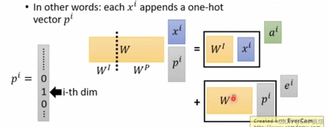
如果正常思维两个ont-hot拼接起来 乘词向量和位置向量矩阵 获取对应的词向量和位置向量 最后的结果跟直接加起来是一样的
假设 token Embedding 矩阵维度是 [200000,768];position Embedding 矩阵维度是 [512,768];segment Embedding ;矩阵维度是 [2,768]。
对于一个token,假设它的 token one-hot 是[1,0,0,0,…0];它的 position one-hot 是[1,0,0,…0];它的 segment one-hot 是[1,0]。那这个token最后的 word Embedding,就是上面三种 Embedding 的加和。如此得到的 word Embedding,和concat后的特征:[1,0,0,0…0,1,0,0…0,1,0],再过维度为 [200000+512+2,768] 的全连接层,得到的向量其实就是一样的。
create_attention_mask_from_input_mask mask矩阵
创建mask矩阵 来找到填充的未知
def create_attention_mask_from_input_mask(from_tensor, to_mask):
  """Create 3D attention mask from a 2D tensor mask.

  Args:
    from_tensor: 2D or 3D Tensor of shape [batch_size, from_seq_length, ...].
    to_mask: int32 Tensor of shape [batch_size, to_seq_length].

  Returns:
    float Tensor of shape [batch_size, from_seq_length, to_seq_length].
  """
  from_shape = get_shape_list(from_tensor, expected_rank=[2, 3])
  batch_size = from_shape[0]
  from_seq_length = from_shape[1]

  to_shape = get_shape_list(to_mask, expected_rank=2)
  to_seq_length = to_shape[1]

  to_mask = tf.cast(
      tf.reshape(to_mask, [batch_size, 1, to_seq_length]), tf.float32)

  # We don't assume that `from_tensor` is a mask (although it could be). We
  # don't actually care if we attend *from* padding tokens (only *to* padding)
  # tokens so we create a tensor of all ones.
  #
  # `broadcast_ones` = [batch_size, from_seq_length, 1]
  broadcast_ones = tf.ones(
      shape=[batch_size, from_seq_length, 1], dtype=tf.float32)

  # Here we broadcast along two dimensions to create the mask.
  #两者想乘 [batch_size,from_seq_length,to_seq_length]
  mask = broadcast_ones * to_mask

  return mask
测试结果
in_a = tf.Variable([[1,2,3,0,0],
                   [4,5,6,7,0]])
mas_a= tf.Variable([[1,1,1,0,0],
                    [1,1,1,1,0]])
result = create_attention_mask_from_input_mask(in_a,mas_a)

结果:
[[[1. 1. 1. 0. 0.]
  [1. 1. 1. 0. 0.]
  [1. 1. 1. 0. 0.]
  [1. 1. 1. 0. 0.]
  [1. 1. 1. 0. 0.]]

 [[1. 1. 1. 1. 0.]
  [1. 1. 1. 1. 0.]
  [1. 1. 1. 1. 0.]
  [1. 1. 1. 1. 0.]
  [1. 1. 1. 1. 0.]]]
attention_layer self_attention层
def attention_layer(from_tensor,
                    to_tensor,
                    attention_mask=None,
                    num_attention_heads=1,
                    size_per_head=512,
                    query_act=None,
                    key_act=None,
                    value_act=None,
                    attention_probs_dropout_prob=0.0,
                    initializer_range=0.02,
                    do_return_2d_tensor=False,
                    batch_size=None,
                    from_seq_length=None,
                    to_seq_length=None):
  """用`from_tensor`(作为Query)去attend to `to_tensor`(提供Key和Value)
	这个函数实现论文"Attention is all you Need"里的multi-head attention。
	如果`from_tensor`和`to_tensor`是同一个tensor,那么就实现Self-Attention。
	`from_tensor`的每个时刻都会attends to `to_tensor`,
        也就是用from的Query去乘以所有to的Key,得到weight,然后把所有to的Value加权求和起来。

	这个函数首先把`from_tensor`变换成一个"query" tensor,
        然后把`to_tensor`变成"key"和"value" tensors。
        总共有`num_attention_heads`组Query、Key和Value,
        每一个Query,Key和Value的shape都是[batch_size(8), seq_length(128), size_per_head(512/8=64)].

	然后计算query和key的内积并且除以size_per_head的平方根(8)。
        然后softmax变成概率,最后用概率加权value得到输出。
        因为有多个Head,每个Head都输出[batch_size, seq_length, size_per_head],
        最后把8个Head的结果concat起来,就最终得到[batch_size(8), seq_length(128), size_per_head*8=512]

	实际上我们是把这8个Head的Query,Key和Value都放在一个Tensor里面的,
        因此实际通过transpose和reshape就达到了上面的效果。

	Args:
		from_tensor: float Tensor,shape [batch_size, from_seq_length, from_width]
		to_tensor: float Tensor,shape [batch_size, to_seq_length, to_width].
		attention_mask: (可选) int32 Tensor, shape[batch_size,from_seq_length,to_seq_length]。
                    值可以是0或者1,在计算attention score的时候,
                    我们会把0变成负无穷(实际是一个绝对值很大的负数),而1不变,
                    这样softmax的时候进行exp的计算,前者就趋近于零,从而间接实现Mask的功能。
		num_attention_heads: int. Attention heads的数量。
		size_per_head: int. 每个head的size
		query_act: (可选) query变换的激活函数
		key_act: (可选) key变换的激活函数
		value_act: (可选) value变换的激活函数
		attention_probs_dropout_prob: (可选) float. attention的Dropout概率。
		initializer_range: float. 初始化范围
		do_return_2d_tensor: bool. 如果True,返回2D的Tensor其shape是
                    [batch_size * from_seq_length, num_attention_heads * size_per_head];
                    否则返回3D的Tensor其shape为[batch_size, from_seq_length,
                                                num_attention_heads * size_per_head].
		batch_size: (可选) int. 如果输入是3D的,那么batch就是第一维,
                    但是可能3D的压缩成了2D的,所以需要告诉函数batch_size
		from_seq_length: (可选) 同上,需要告诉函数from_seq_length
		to_seq_length: (可选) 同上,to_seq_length

	Returns:
		float Tensor,shape [batch_size,from_seq_length,num_attention_heads * size_per_head]。
		如果`do_return_2d_tensor`为True,则返回的shape是
                       [batch_size * from_seq_length, num_attention_heads * size_per_head]
  """

  def transpose_for_scores(input_tensor, batch_size, num_attention_heads,
                           seq_length, width):
    output_tensor = tf.reshape(
        input_tensor, [batch_size, seq_length, num_attention_heads, width])


  # tf.transpose  表示进行转置操作   第二份参数表示shape 例如原来【3,4,5】  经过
    # tf.transpose(output_tensor, [0, 2, 1]) 则变成了【3,5,4】
    output_tensor = tf.transpose(output_tensor, [0, 2, 1, 3])
    return output_tensor

  from_shape = get_shape_list(from_tensor, expected_rank=[2, 3])
  to_shape = get_shape_list(to_tensor, expected_rank=[2, 3])

  if len(from_shape) != len(to_shape):
    raise ValueError(
        "The rank of `from_tensor` must match the rank of `to_tensor`.")

  # 如果输入是3D的(没有压缩),那么我们可以推测出batch_size、from_seq_length和to_seq_length
	# 即使参数传入也会被覆盖。
  if len(from_shape) == 3:
    batch_size = from_shape[0]
    from_seq_length = from_shape[1]
    to_seq_length = to_shape[1]
  elif len(from_shape) == 2:
      #如果输入时2维的  则要都说清楚
    if (batch_size is None or from_seq_length is None or to_seq_length is None):
      raise ValueError(
          "When passing in rank 2 tensors to attention_layer, the values "
          "for `batch_size`, `from_seq_length`, and `to_seq_length` "
          "must all be specified.")

  # Scalar dimensions referenced here:
  #   B = batch size (number of sequences)
  #   F = `from_tensor` sequence length
  #   T = `to_tensor` sequence length
  #   N = `num_attention_heads`
  #   H = `size_per_head`

 #本来是二维 所以不变
  # [batch_size*length,width]
  from_tensor_2d = reshape_to_matrix(from_tensor)
  to_tensor_2d = reshape_to_matrix(to_tensor)

  # `query_layer` = [B*F, N*H]
  # 计算Query `query_layer` = [B*F, N*H] =[8*128, 12*64]
  # batch_size=8,共128个时刻,12和head,每个head的query向量是64
  # 因此最终得到[8*128, 12*64]
  query_layer = tf.layers.dense(
      from_tensor_2d,
      num_attention_heads * size_per_head,
      activation=query_act,
      name="query",
      kernel_initializer=create_initializer(initializer_range))

  # `key_layer` = [B*T, N*H]
  #因此最终得到[8 * 128, 12 * 64]
  key_layer = tf.layers.dense(
      to_tensor_2d,
      num_attention_heads * size_per_head,
      activation=key_act,
      name="key",
      kernel_initializer=create_initializer(initializer_range))

  # `value_layer` = [B*T, N*H]
  #因此最终得到[8*128, 12*64]
  value_layer = tf.layers.dense(
      to_tensor_2d,
      num_attention_heads * size_per_head,
      activation=value_act,
      name="value",
      kernel_initializer=create_initializer(initializer_range))

  # `query_layer` = [B, N, F, H]
  # 把query从[B*F, N*H] =[8*128, 12*64]变成[B, N, F, H]=[8, 12, 128, 64]
  query_layer = transpose_for_scores(query_layer, batch_size,
                                     num_attention_heads, from_seq_length,
                                     size_per_head)

  # `key_layer` = [B, N, T, H]
  # 从[B*F, N*H] =[8*128, 12*64]变成[B, N, F, H]=[8, 12, 128, 64]
  key_layer = transpose_for_scores(key_layer, batch_size, num_attention_heads,
                                   to_seq_length, size_per_head)

  # Take the dot product between "query" and "key" to get the raw
  # attention scores.
  # `attention_scores` = [B, N, F, T]
  # 计算query和key的内积,得到attention scores.
  # [8, 12, 128, 64]*[8, 12, 64, 128]=[8, 12, 128, 128]
  # 最后两维[128, 128]表示from的128个时刻attend to到to的128个score。
  #transpose_b  b发生转置
  attention_scores = tf.matmul(query_layer, key_layer, transpose_b=True)
  attention_scores = tf.multiply(attention_scores,
                                 1.0 / math.sqrt(float(size_per_head)))

  # mask的用法是在softmax之前加起来   如果mask是1 0  如果是0  就是一个很小的负数
  if attention_mask is not None:
    # `attention_mask` = [B, 1, F, T]
    # 从[8, 128, 128]变成[8, 1, 128, 128]
    # `attention_mask` = [B, 1, F, T]
    #  在某一维进行扩充
    attention_mask = tf.expand_dims(attention_mask, axis=[1])

    # 这个小技巧前面也用到过,如果mask是1,那么(1-1)*-10000=0,adder就是0,
    # 如果mask是0,那么(1-0)*-10000=-10000。
    adder = (1.0 - tf.cast(attention_mask, tf.float32)) * -10000.0

    # 我们把adder加到attention_score里,mask是1就相当于加0,mask是0就相当于加-10000。
    # 通常attention_score都不会很大,因此mask为0就相当于把attention_score设置为负无穷
    # 后面softmax的时候就趋近于0,因此相当于不能attend to Mask为0的地方。
    attention_scores += adder

  # Normalize the attention scores to probabilities.
  # `attention_probs` = [B, N, F, T]
  attention_probs = tf.nn.softmax(attention_scores)

  # This is actually dropping out entire tokens to attend to, which might
  # seem a bit unusual, but is taken from the original Transformer paper.
  attention_probs = dropout(attention_probs, attention_probs_dropout_prob)

  # `value_layer` = [B, T, N, H]
  #把`value_layer` reshape成[B, T, N, H]=[8, 128, 12, 64]
  value_layer = tf.reshape(
      value_layer,
      [batch_size, to_seq_length, num_attention_heads, size_per_head])

  # `value_layer` = [B, N, T, H]
  # `value_layer`变成[B, N, T, H]=[8, 12, 128, 64]
  value_layer = tf.transpose(value_layer, [0, 2, 1, 3])

  # `context_layer` = [B, N, F, H]
  # 计算`context_layer` = [8, 12, 128, 128]*[8, 12, 128, 64]=[8, 12, 128, 64]=[B, N, F, H]
  context_layer = tf.matmul(attention_probs, value_layer)

  # `context_layer` = [B, F, N, H]

  # `context_layer` 变换成 [B, F, N, H]=[8, 128, 12, 64]
  context_layer = tf.transpose(context_layer, [0, 2, 1, 3])

  if do_return_2d_tensor:
      # 默认true
    # `context_layer` = [B*F, N*H]
    context_layer = tf.reshape(
        context_layer,
        [batch_size * from_seq_length, num_attention_heads * size_per_head])
  else:
    # `context_layer` = [B, F, N*H]
    context_layer = tf.reshape(
        context_layer,
        [batch_size, from_seq_length, num_attention_heads * size_per_head])

  return context_layer
计算逻辑
Attention层计算逻辑(多头机制)
原始输入                     from_tensor [batch_size,length,width]         to_tensor [batch_size,length,width]
为了计算转换                  from_tensor [batch_size*length,width]         to_tensor [batch_size*length,width]
利用tf.laysers.dense实现多头  Q [batch_size*length,head_num*head_size]      K [batch_size*length,head_num*head_size]    V [batch_size*length,head_num*head_size]
转换一下                     Q [batch_size,head_num,length,head_size]      K [batch_size,head_num,head_size,length]    V [batch_size,head_num,length,head_size]
Q和K矩阵乘积   tf.matul(Q,K)  [batch_size,head_num,length,length]
softmax后与V乘积              [batch_size,head_num,length,head_size]
转换                         [batch_size,length,head_num*head_size]
为什么使用不同的Q,K,而不是使用同一个
想要回答这个问题,我们首先要明白,为什么要计算Q和K的点乘。现补充两点先从点乘的物理意义说,1. 两个向量的点乘表示两个向量的相似度。
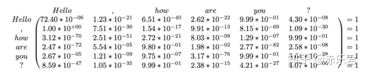
2. Q,K,V物理意义上是一样的,都表示同一个句子中不同token组成的矩阵。矩阵中的每一行,是表示一个token的word embedding向量。假设一个句子"Hello, how are you?"长度是6,embedding维度是300,那么Q,K,V都是(6, 300)的矩阵简单的说,K和Q的点乘是为了计算一个句子中每个token相对于句子中其他token的相似度,这个相似度可以理解为attetnion score,关注度得分。比如说 "Hello, how are you?"这句话,当前token为”Hello"的时候,我们可以知道”Hello“对于” , “, “how”, “are”, “you”, "?"这几个token对应的关注度是多少。有了这个attetnion score,可以知道处理到”Hello“的时候,模型在关注句子中的哪些token。
赤乐君
这个attention score是一个(6, 6)的矩阵。每一行代表每个token相对于其他token的关注度。比如说上图中的第一行,代表的是Hello这个单词相对于本句话中的其他单词的关注度。添加softmax只是为了对关注度进行归一化。虽然有了attention score矩阵,但是这个矩阵是经过各种计算后得到的,已经很难表示原来的句子了。然而V还代表着原来的句子,所以我们拿这个attention score矩阵与V相乘,得到的是一个加权后结果。也就是说,原本V里的各个单词只用word embedding表示,相互之间没什么关系。但是经过与attention score相乘后,V中每个token的向量(即一个单词的word embedding向量),在300维的每个维度上(每一列)上,都会对其他token做出调整(关注度不同)。与V相乘这一步,相当于提纯,让每个单词关注该关注的部分。
好了,该解释为什么不把K和Q用同一个值了。经过上面的解释,我们知道K和Q的点乘是为了得到一个attention score 矩阵,用来对V进行提纯。K和Q使用了不同的W_k, W_Q来计算,可以理解为是在不同空间上的投影。正因为有了这种不同空间的投影,增加了表达能力,这样计算得到的attention score矩阵的泛化能力更高。这里解释下我理解的泛化能力,因为K和Q使用了不同的W_k, W_Q来计算,得到的也是两个完全不同的矩阵,所以表达能力更强。但是如果不用Q,直接拿K和K点乘的话,你会发现attention score 矩阵是一个对称矩阵。因为是同样一个矩阵,都投影到了同样一个空间,所以泛化能力很差。这样的矩阵导致对V进行提纯的时候,效果也不会好。
多头的计算逻辑(代码也有体现)
BERT由12层transformer layer(encoder端)构成,首先word emb , pos emb(可能会被问到有哪几种position embedding的方式,bert是使用的哪种), sent emb做加和作为网络输入,每层由一个multi-head attention, 一个feed forward 以及两层layerNorm构成,一般会被问到multi-head attention的结构,具体可以描述为,
- step1一个768的hidden向量,被映射成query, key, value。 然后三个向量分别切分成12个小的64维的向量,每一组小向量之间做attention。不妨假设batch_size为32,seqlen为512,隐层维度为768,12个head,
hidden(32 x 512 x 768) -> query(32 x 512 x 768) -> 32 x 12 x 512 x 64
hidden(32 x 512 x 768) -> key(32 x 512 x 768) -> 32 x 12 x 512 x 64
hidden(32 x 512 x 768) -> val(32 x 512 x 768) -> 32 x 12 x 512 x 64
最后一步是多头的体现 - step2然后query和key之间做attention,得到一个32 x 12 x 512 x 512的权重矩阵,然后根据这个权重矩阵加权value中切分好的向量,得到一个32 x 12 x 512 x 64 的向量,拉平输出为768向量。
32 x 12 x 512 x 64(query_hidden) * 32 x 12 x 64 x 512(key_hidden) -> 32 x 12 x 512 x 512
32 x 12 x 64 x 512(value_hidden) * 32 x 12 x 512 x 512 (权重矩阵) -> 32 x 12 x 512 x 64
然后再还原成 -> 32 x 512 x 768
简言之是12个头,每个头都是一个64维度分别去与其他的所有位置的hidden embedding做attention然后再合并还原。
transformer_model层
def transformer_model(input_tensor,
                      attention_mask=None,
                      hidden_size=768,
                      num_hidden_layers=12,
                      num_attention_heads=12,
                      intermediate_size=3072,
                      intermediate_act_fn=gelu,
                      hidden_dropout_prob=0.1,
                      attention_probs_dropout_prob=0.1,
                      initializer_range=0.02,
                      do_return_all_layers=False):
  """Multi-headed, multi-layer的Transformer,参考"Attention is All You Need".

  这基本上是和原始Transformer encoder相同的代码。

  原始论文为:
  https://arxiv.org/abs/1706.03762

  Also see:
  https://github.com/tensorflow/tensor2tensor/blob/master/tensor2tensor/models/transformer.py

  Args:
    input_tensor: float Tensor,shape为[batch_size, seq_length, hidden_size]
    attention_mask: (可选) int32 Tensor,shape [batch_size, seq_length,
      seq_length], 1表示可以attend to,0表示不能。
    hidden_size: int. Transformer隐单元个数
    num_hidden_layers: int. 有多少个SubLayer
    num_attention_heads: int. Transformer Attention Head个数。
    intermediate_size: int. 全连接层的隐单元个数
    intermediate_act_fn: 函数. 全连接层的激活函数。
    hidden_dropout_prob: float. Self-Attention层残差之前的Dropout概率
    attention_probs_dropout_prob: float. attention的Dropout概率
    initializer_range: float. 初始化范围(truncated normal的标准差)
    do_return_all_layers: 返回所有层的输出还是最后一层的输出。

  Returns:
    如果do_return_all_layers True,返回最后一层的输出,是一个Tensor,
                shape为[batch_size, seq_length, hidden_size];
    否则返回所有层的输出,是一个长度为num_hidden_layers的list,
                list的每一个元素都是[batch_size, seq_length, hidden_size]。

  """
  if hidden_size % num_attention_heads != 0:
    raise ValueError(
        "The hidden size (%d) is not a multiple of the number of attention "
        "heads (%d)" % (hidden_size, num_attention_heads))

 #因为最终要输出hidden_size,总共有num_attention_heads个Head,因此每个Head输出
  # 为hidden_size / num_attention_heads
  attention_head_size = int(hidden_size / num_attention_heads)
  input_shape = get_shape_list(input_tensor, expected_rank=3)
  batch_size = input_shape[0]
  seq_length = input_shape[1]
  input_width = input_shape[2]

  # The Transformer performs sum residuals on all layers so the input needs
  # to be the same as the hidden size.
  if input_width != hidden_size:
    raise ValueError("The width of the input tensor (%d) != hidden size (%d)" %
                     (input_width, hidden_size))

  # We keep the representation as a 2D tensor to avoid re-shaping it back and
  # forth from a 3D tensor to a 2D tensor. Re-shapes are normally free on
  # the GPU/CPU but may not be free on the TPU, so we want to minimize them to
  # help the optimizer.
  # 为了避免在2D和3D之间来回reshape,我们统一把所有的3D Tensor用2D来表示。
  # 虽然reshape在GPU/CPU上很快,但是在TPU上却不是这样,这样做的目的是为了优化TPU
  # input_tensor是[8, 128, 768], prev_output是[8*128, 768]=[1024, 768]
  prev_output = reshape_to_matrix(input_tensor)

  all_layer_outputs = []


  #12层的attention
  #  每一层都有两个残差神经网络,那每一层的输出 放到一个list里面
  for layer_idx in range(num_hidden_layers):
    with tf.variable_scope("layer_%d" % layer_idx):

      #prev_output是[8*128, 768]=[1024, 768]
      layer_input = prev_output

      with tf.variable_scope("attention"):
        attention_heads = []
        with tf.variable_scope("self"):
          attention_head = attention_layer(
              from_tensor=layer_input,
              to_tensor=layer_input,
              attention_mask=attention_mask,
              num_attention_heads=num_attention_heads,
              size_per_head=attention_head_size,
              attention_probs_dropout_prob=attention_probs_dropout_prob,
              initializer_range=initializer_range,
              do_return_2d_tensor=True,
              batch_size=batch_size,
              from_seq_length=seq_length,
              to_seq_length=seq_length)
          # 返回是 [batch_size * from_seq_length, num_attention_heads * size_per_head])
          attention_heads.append(attention_head)

        attention_output = None
        if len(attention_heads) == 1:
          attention_output = attention_heads[0]
        else:
          # In the case where we have other sequences, we just concatenate
          # them to the self-attention head before the projection.
          attention_output = tf.concat(attention_heads, axis=-1)

        # Run a linear projection of `hidden_size` then add a residual
        # with `layer_input`.
        #  添加前项神经 网路  加了残差
        with tf.variable_scope("output"):
          attention_output = tf.layers.dense(
              attention_output,
              hidden_size,
              kernel_initializer=create_initializer(initializer_range))
          attention_output = dropout(attention_output, hidden_dropout_prob)
          # 残差神经网络
          attention_output = layer_norm(attention_output + layer_input)

      # The activation is only applied to the "intermediate" hidden layer.
      #  增加非线性 feed-forward层
      with tf.variable_scope("intermediate"):
        intermediate_output = tf.layers.dense(
            attention_output,
            intermediate_size,
            activation=intermediate_act_fn,
            kernel_initializer=create_initializer(initializer_range))

      # Down-project back to `hidden_size` then add the residual.
      #对前面的输出进行一个线性转换  hidden_size   加上残差
      with tf.variable_scope("output"):
        layer_output = tf.layers.dense(
            intermediate_output,
            hidden_size,
            kernel_initializer=create_initializer(initializer_range))
        layer_output = dropout(layer_output, hidden_dropout_prob)

        # 残差神经网络
        layer_output = layer_norm(layer_output + attention_output)
        prev_output = layer_output
        all_layer_outputs.append(layer_output)

  if do_return_all_layers:
    final_outputs = []
    for layer_output in all_layer_outputs:
      final_output = reshape_from_matrix(layer_output, input_shape)
      final_outputs.append(final_output)
    return final_outputs
  else:
    final_output = reshape_from_matrix(prev_output, input_shape)
    return final_output
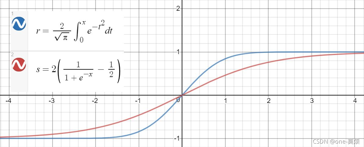
GELU激活函数
在原始论文中,给出了两种近似的表达
Sigmoid近似:
![[公式]](https://i-blog.csdnimg.cn/blog_migrate/e0a6755f9ca338134f06fd4d1d14ed9a.png)
,其图像如下:
另一种是tanh近似

其图像如下
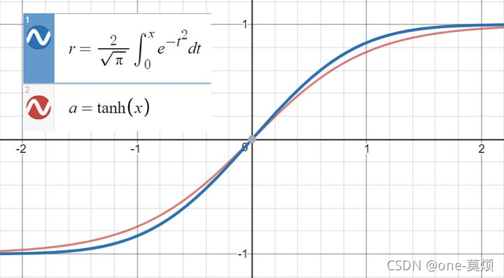
在 bert中用的是tanh近似 ,原始代码如下
def gelu(x):
  """Gaussian Error Linear Unit.

  This is a smoother version of the RELU.
  Original paper: https://arxiv.org/abs/1606.08415
  Args:
    x: float Tensor to perform activation.

  Returns:
    `x` with the GELU activation applied.
  """
  cdf = 0.5 * (1.0 + tf.tanh(
      (np.sqrt(2 / np.pi) * (x + 0.044715 * tf.pow(x, 3)))))
  return x * cdf
BertModel类
class BertModel(object):
  """BERT model ("Bidirectional Encoder Representations from Transformers").

  Example usage:

  ```python
  # Already been converted into WordPiece token ids
  input_ids = tf.constant([[31, 51, 99], [15, 5, 0]])
  input_mask = tf.constant([[1, 1, 1], [1, 1, 0]])
  token_type_ids = tf.constant([[0, 0, 1], [0, 2, 0]])

  config = modeling.BertConfig(vocab_size=32000, hidden_size=512,
    num_hidden_layers=8, num_attention_heads=6, intermediate_size=1024)

  model = modeling.BertModel(config=config, is_training=True,
    input_ids=input_ids, input_mask=input_mask, token_type_ids=token_type_ids)

  label_embeddings = tf.get_variable(...)
  pooled_output = model.get_pooled_output()
  logits = tf.matmul(pooled_output, label_embeddings)
  """

  def __init__(self,
               config,
               is_training,
               input_ids,
               input_mask=None,
               token_type_ids=None,
               use_one_hot_embeddings=False,
               scope=None):
    """Constructor for BertModel.
    # Args:
  #       config: `BertConfig` 对象
  #       is_training: bool 表示训练还是eval,是会影响dropout
  #	  input_ids: int32 Tensor  shape是[batch_size, seq_length]
  #	  input_mask: (可选) int32 Tensor shape是[batch_size, seq_length]
  #	  token_type_ids: (可选) int32 Tensor shape是[batch_size, seq_length]
  #	  use_one_hot_embeddings: (可选) bool
  #		  如果True,使用矩阵乘法实现提取词的Embedding;否则用tf.embedding_lookup()
  #		  对于TPU,使用前者更快,对于GPU和CPU,后者更快。
  #	  scope: (可选) 变量的scope。默认是"bert"

  # Raises:
  #	  ValueError: 如果config或者输入tensor的shape有问题就会抛出这个异常
    """
    config = copy.deepcopy(config)
    if not is_training:
      config.hidden_dropout_prob = 0.0
      config.attention_probs_dropout_prob = 0.0

    #[batch_size, seq_length]
    input_shape = get_shape_list(input_ids, expected_rank=2)
    batch_size = input_shape[0]
    seq_length = input_shape[1]

    if input_mask is None:
        #  没有mask  那就全部都是1  主要是人为填补 补齐用的
      input_mask = tf.ones(shape=[batch_size, seq_length], dtype=tf.int32)

    if token_type_ids is None:
        #  没有上下文 则全部为0
      token_type_ids = tf.zeros(shape=[batch_size, seq_length], dtype=tf.int32)

    with tf.variable_scope(scope, default_name="bert"):
      with tf.variable_scope("embeddings"):
        # Perform embedding lookup on the word ids.
        # 每一个词的embeding
        # [batch_size,length,vocab_size]
        (self.embedding_output, self.embedding_table) = embedding_lookup(
            input_ids=input_ids,
            vocab_size=config.vocab_size,
            embedding_size=config.hidden_size,
            initializer_range=config.initializer_range,
            word_embedding_name="word_embeddings",
            use_one_hot_embeddings=use_one_hot_embeddings)

        # Add positional embeddings and token type embeddings, then layer
        # normalize and perform dropout.
        # 加上 位置  语句信息
        self.embedding_output = embedding_postprocessor(
            input_tensor=self.embedding_output,
            use_token_type=True,
            token_type_ids=token_type_ids,
            token_type_vocab_size=config.type_vocab_size,
            token_type_embedding_name="token_type_embeddings",
            use_position_embeddings=True,
            position_embedding_name="position_embeddings",
            initializer_range=config.initializer_range,
            max_position_embeddings=config.max_position_embeddings,
            dropout_prob=config.hidden_dropout_prob)

      with tf.variable_scope("encoder"):
        # 把shape为[batch_size, seq_length]的2D mask变成
        # shape为[batch_size, seq_length, seq_length]的3D mask
        # 返回batch_size个  mask矩阵 每一个是【seq_len,seq_len】
        #v注意[batch, A, B]*[batch, B, C]=[batch, A, C],
        # 我们可以认为是batch个[A, B]的矩阵乘以batch个[B, C]的矩阵。
        #这个主要是减少对于mask的词和填充部分的词的关注。mask部分和填充部分在计算attention的时候分数自然应该很低才对。
        attention_mask = create_attention_mask_from_input_mask(
            input_ids, input_mask)

        # Run the stacked transformer.
        # `sequence_output` shape = [batch_size, seq_length, hidden_size].
        # all_encoder_layers是一个list,长度为num_hidden_layers(默认12),每一层对应一个值。
        # 每一个值都是一个shape为[batch_size, seq_length, hidden_size]的tensor。
        self.all_encoder_layers = transformer_model(
            input_tensor=self.embedding_output,
            attention_mask=attention_mask,
            hidden_size=config.hidden_size,
            num_hidden_layers=config.num_hidden_layers,
            num_attention_heads=config.num_attention_heads,
            intermediate_size=config.intermediate_size,
            intermediate_act_fn=get_activation(config.hidden_act),
            hidden_dropout_prob=config.hidden_dropout_prob,
            attention_probs_dropout_prob=config.attention_probs_dropout_prob,
            initializer_range=config.initializer_range,
            do_return_all_layers=True)

      #获取最后一层的结果 shape是[batch_size, seq_length, hidden_size]
      self.sequence_output = self.all_encoder_layers[-1]

      # 取最后一层的第一个时刻[CLS]对应的tensor
      # 从[batch_size, seq_length, hidden_size]变成[batch_size, hidden_size]
      # sequence_output[:, 0:1, :]得到的是[batch_size, 1, hidden_size]
      # 我们需要用squeeze把第二维去掉。
      with tf.variable_scope("pooler"):
        # tf.squeeze  去掉维度为1的
        first_token_tensor = tf.squeeze(self.sequence_output[:, 0:1, :], axis=1)
        self.pooled_output = tf.layers.dense(
            first_token_tensor,
            config.hidden_size,
            activation=tf.tanh,
            kernel_initializer=create_initializer(config.initializer_range))

  def get_pooled_output(self):
    return self.pooled_output

  def get_sequence_output(self):
    """Gets final hidden layer of encoder.

    Returns:
      float Tensor of shape [batch_size, seq_length, hidden_size] corresponding
      to the final hidden of the transformer encoder.
    """
    return self.sequence_output

  def get_all_encoder_layers(self):
    return self.all_encoder_layers

  def get_embedding_output(self):
    """Gets output of the embedding lookup (i.e., input to the transformer).

    Returns:
      float Tensor of shape [batch_size, seq_length, hidden_size] corresponding
      to the output of the embedding layer, after summing the word
      embeddings with the positional embeddings and the token type embeddings,
      then performing layer normalization. This is the input to the transformer.
    """
    return self.embedding_output

  def get_embedding_table(self):
    return self.embedding_table
LayerNorm详解
class BertLayerNorm(nn.Module):
    def __init__(self, hidden_size, eps=1e-5):
        super(BertLayerNorm, self).__init__()
        self.weight = nn.Parameter(torch.ones(hidden_size))
        self.bias = nn.Parameter(torch.zeros(hidden_size))
        self.variance_epsilon = eps

    def forward(self, x):
        u = x.mean(-1, keepdim=True)
        s = (x - u).pow(2).mean(-1, keepdim=True)
        x = (x - u) / torch.sqrt(s + self.variance_epsilon)
        return self.weight * x + self.bias
LayerNorm则是针对单个样本,不依赖于其他数据,常被用于小mini-batch场景、动态网络场景和 RNN,特别是自然语言处理领域,就bert来说就是对每层输出的隐层向量(768维)做规范化。
其实可以发现在规范话后又加了weight和bias,这样的目的是?
参考百面机器学习220-221页,为了搞清楚为什么归一化层有一个w,b这两个参数归一化是为了让本层网络的输出进行额外的约束,但如果每个网络的输出被限制在这个约束内,就会限制模型的表达能力。 通俗的讲,不管你上层网络输出的是什么牛鬼蛇神的向量,都先给我归一化到正态分布(均值为0,标准差为1),但我不能给下游传这个向量,如果这样下游网络看到的只能是归一化后的,限制了模型。(先归一化,在适当还原成下游网络合适的分布,通过模型学习)
链接:知乎。
wordpiece
wordpiece其核心思想是将单词打散为字符,然后根据片段的组合频率,最后单词切分成片段处理。
WordPiece的一种主要的实现方式叫做BPE(Byte-Pair Encoding)双字节编码。
BPE的过程可以理解为把一个单词再拆分,使得我们的此表会变得精简,并且寓意更加清晰。
比如"loved",“loving”,"loves"这三个单词。其实本身的语义都是“爱”的意思,但是如果我们以单词为单位,那它们就算不一样的词,在英语中不同后缀的词非常的多,就会使得词表变的很大,训练速度变慢,训练的效果也不是太好。
BPE算法通过训练,能够把上面的3个单词拆分成"lov",“ed”,“ing”,"es"几部分,这样可以把词的本身的意思和时态分开,有效的减少了词表的数量。
具体是怎么做分词的??
Bert分词
对于中文来说只有BasicTokenizer 英文除了BasicTokenizer还有WordpieceTokenizer
BasicTokenizer
example = "Keras是ONEIROS(Open-ended Neuro-Electronic Intelligent Robot Operating System,开放式神经电子智能机器人操作系统)项目研究工作
		  的部分产物[3],主要作者和维护者是Google工程师François Chollet。\r\n"
(1)转成unicode
	主要是对python3、2的不同输入做处理,经过这步后 例子不变
	example = "Keras是ONEIROS(Open-ended Neuro-Electronic Intelligent Robot Operating System,开放式神经电子智能机器人操作系统)项目研究工作
		  的部分产物[3],主要作者和维护者是Google工程师François Chollet。\r\n"
(2)去处各种奇怪字符
	去除各种不合法字符和多余空格   经过这步后,example 中的 \r\n 被替换成两个空格:
			 'Keras是ONEIROS(Open-ended Neuro-Electronic Intelligent Robot Operating System,开放式神经电子智能机器人操作系统)项目研究工作
			 的部分产物[3],主要作者和维护者是Google工程师François Chollet。  '
(3)处理中文
	 首先判断其是不是「中文字符」(关于中文字符的说明见下方引用块说明),是的话在其前后加上一个空格,否则原样输出。 经过这步后,中文被按字分
	 开,用空格分隔,但英文数字等仍然保持原状
			 'Keras 是 ONEIROS(Open-ended Neuro-Electronic Intelligent Robot Operating System, 开  放  式  神  经  电  子  智  能  机  器  人  操  作  系  统 )
				 项  目  研  究  工  作  的  部  分  产  物 [3], 主  要  作  者  和  维  护  者  是 Google 工  程  师 François Chollet。  '

(4)空格分词
	  首先对 text 进行 strip() 操作,去掉两边多余空白字符,然后如果剩下的是一个空字符串,则直接返回空列表,否则进行 split() 操作,得到最初的分词结果
['Keras', '是', 'ONEIROS(Open-ended', 'Neuro-Electronic', 'Intelligent', 'Robot', 'Operating', 'System,', '开', '放', '式', '神', '经', '电', '子',
 '智', '能', '机', '器', '人', '操', '作', '系', '统', ')', '项', '目', '研', '究', '工', '作', '的', '部', '分', '产', '物', '[3],', '主', '要', '作',
 '者', '和', '维', '护', '者', '是', 'Google', '工', '程', '师', 'François', 'Chollet。']
(5)去除多余字符和标点分词
	  用于去除变音符号  经过这步后,原先没有被分开的字词标点(例如 ONEIROS(Open-ended)、没有去掉的变音符号(例如 ç)都被相应处理:
['keras', '是', 'oneiros', '(', 'open', '-', 'ended', 'neuro', '-', 'electronic', 'intelligent', 'robot', 'operating', 'system', ',', '开', '放', '式',
  '神', '经', '电', '子', '智', '能', '机', '器', '人', '操', '作', '系', '统', ')', '项', '目', '研', '究', '工', '作', '的', '部', '分', '产', '物',
  '[', '3', ']', ',', '主', '要', '作', '者', '和', '维', '护', '者', '是', 'google', '工', '程', '师', 'francois', 'chollet', '。']
(6)再次空格分词
['keras', '是', 'oneiros', '(', 'open', '-', 'ended', 'neuro', '-', 'electronic', 'intelligent', 'robot', 'operating', 'system', ',', '开', '放', '式',
  '神', '经', '电', '子', '智', '能', '机', '器', '人', '操', '作', '系', '统', ')', '项', '目', '研', '究', '工', '作', '的', '部', '分', '产', '物',
  '[', '3', ']', ',', '主', '要', '作', '者', '和', '维', '护', '者', '是', 'google', '工', '程', '师', 'francois', 'chollet', '。']
WordpieceTokenizer
首先读取一个词表(包含所有的字词),分词思路是按照从左到右的顺序,将一个词拆分成多个子词,每个子词尽可能长。
用unaffable举例子
1 从第一个位置开始,由于是最长匹配,结束位置需要从最右端依次递减,所以遍历的第一个子词是其本身 unaffable,该子词不在词汇表中
2 结束位置左移一位得到子词 unaffabl,同样不在词汇表中
3 重复这个操作,直到 un,该子词在词汇表中,将其加入 output_tokens,以第一个位置开始的遍历结束
4 跳过 un,从其后的 a 开始新一轮遍历,结束位置依然是从最右端依次递减,但此时需要在前面加上 ## 标记,得到 ##affable 不在词汇表中
6 结束位置左移一位得到子词 ##affabl,同样不在词汇表中
7 重复这个操作,直到 ##aff,该字词在词汇表中,将其加入 output_tokens,此轮遍历结束
8 跳过 aff,从其后的 a 开始新一轮遍历,结束位置依然是从最右端依次递减。##able 在词汇表中,将其加入 output_tokens
9 able 后没有字符了,整个遍历结束

  ['keras', '是', 'one', '##iros', '(', 'open', '-', 'ended', 'neu', '##ro', '-', 'electronic', 'intelligent', 'robot', 'operating', 'system', ',', '开', '放',
  '式', '神', '经', '电', '子', '智', '能', '机', '器', '人', '操', '作', '系', '统', ')', '项', '目', '研', '究', '工', '作', '的', '部', '分', '产', '物',
  '[', '3', ']', ',', '主', '要', '作', '者', '和', '维', '护', '者', '是', 'google', '工', '程', '师', 'franco', '##is', 'cho', '##llet', '。']
bert是如何做warm-up和decay?
上代码
  global_step = tf.train.get_or_create_global_step()

  # 专门用于 bert层更新的学习率
  bert_learning_rate = tf.constant(value=bert_lr, shape=[], dtype=tf.float32)
  # Implements linear decay of the learning rate.
  # 最终会衰减到0
  bert_learning_rate = tf.train.polynomial_decay(
      bert_learning_rate,
      global_step,
      num_train_steps,
      end_learning_rate=0.0,
      power=1.0,
      cycle=False)
  # Implements linear warmup. I.e., if global_step < num_warmup_steps, the
  # learning rate will be `global_step/num_warmup_steps * init_lr`.
  # 在热身的时候  学习率是一个线性增长的趋势   然后就是学习率衰减了
  if num_warmup_steps:
      global_steps_int = tf.cast(global_step, tf.int32)
      warmup_steps_int = tf.constant(num_warmup_steps, dtype=tf.int32)

      global_steps_float = tf.cast(global_steps_int, tf.float32)
      warmup_steps_float = tf.cast(warmup_steps_int, tf.float32)

      #  当前的步数 / 热身需要的步数
      warmup_percent_done = global_steps_float / warmup_steps_float
      warmup_learning_rate = bert_lr * warmup_percent_done
      # 判断热身的步数 和 设定的部署之间的关系
      is_warmup = tf.cast(global_steps_int < warmup_steps_int, tf.float32)
      bert_learning_rate = (
              (1.0 - is_warmup) * bert_learning_rate + is_warmup * warmup_learning_rate)
  # It is recommended that you use this optimizer for fine tuning, since this
  # is how the model was trained (note that the Adam m/v variables are NOT
  # loaded from init_checkpoint.)
  bert_optimizer = AdamWeightDecayOptimizer(
      learning_rate=bert_learning_rate,
      weight_decay_rate=0.01,
      beta_1=0.9,
      beta_2=0.999,
      epsilon=1e-6,
      exclude_from_weight_decay=["LayerNorm", "layer_norm", "bias"])
学习率会在热身的步长单位内线性增长 当达到热身步长的时候 在使用decay 然后衰减
这么做的原因?
这是因为,刚开始模型对数据的“分布”理解为零,或者是说“均匀分布”(当然这取决于你的初始化);在第一轮训练的时候,每个数据点对模型来说都是新的,模型会很快地进行数据分布修正,如果这时候学习率就很大,极有可能导致开始的时候就对该数据“过拟合”,后面要通过多轮训练才能拉回来,浪费时间。当训练了一段时间(比如两轮、三轮)后,模型已经对每个数据点看过几遍了,或者说对当前的batch而言有了一些正确的先验,较大的学习率就不那么容易会使模型学偏,所以可以适当调大学习率。这个过程就可以看做是warmup。那么为什么之后还要decay呢?当模型训到一定阶段后(比如十个epoch),模型的分布就已经比较固定了,或者说能学到的新东西就比较少了。如果还沿用较大的学习率,就会破坏这种稳定性,用我们通常的话说,就是已经接近loss的local optimal了,为了达到最优解,学习率必须很小。
bert预训练任务
Masked Language Model(MLM)
MLM是BERT能够不受单向语言模型所限制的原因。简单来说就是以15%的概率用mask token ([MASK])随机地对每一个训练序列中的token进行替换,然后预测出[MASK]位置原有的单词。然而,由于[MASK]并不会出现在下游任务的微调(fine-tuning)阶段,因此预训练阶段和微调阶段之间产生了不匹配(这里很好解释,就是预训练的目标会令产生的语言表征对[MASK]敏感,但是却对其他token不敏感)。因此BERT采用了以下策略来解决这个问题:
首先在每一个训练序列中以15%的概率随机地选中某个token位置用于预测,假如是第i个token被选中,则会被替换成以下三个token之一
1)80%的时候是[MASK]。如,my dog is hairy——>my dog is [MASK]
2)10%的时候是随机的其他token。如,my dog is hairy——>my dog is apple
3)10%的时候是原来的token(保持不变,个人认为是作为2)所对应的负类)。如,my dog is hairy——>my dog is hairy
再用该位置对应的 T_i去预测出原来的token(输入到全连接,然后用softmax输出每个token的概率,最后用交叉熵计算loss)。该策略令到BERT不再只对[MASK]敏感,而是对所有的token都敏感,以致能抽取出任何token的表征信息。
Next Sentence Prediction(NSP)
一些如问答、自然语言推断等任务需要理解两个句子之间的关系,而MLM任务倾向于抽取token层次的表征,因此不能直接获取句子层次的表征。为了使模型能够有能力理解句子间的关系,BERT使用了NSP任务来预训练,简单来说就是预测两个句子是否连在一起。具体的做法是:对于每一个训练样例,我们在语料库中挑选出句子A和句子B来组成,50%的时候句子B就是句子A的下一句(标注为IsNext),剩下50%的时候句子B是语料库中的随机句子(标注为NotNext)。接下来把训练样例输入到BERT模型中,用[CLS]对应的C信息去进行二分类的预测。
bert预训练中的损失函数
BERT的损失函数由两部分组成,第一部分是来自 MLM 的单词级别分类任务,另一部分是来自NSP的句子级别的分类任务。通过这两个任务的联合学习(是同时训练,而不是前后训练),可以使得 BERT 学习到的表征既有 token 级别信息,同时也包含了句子级别的语义信息。
具体损失函数如下:

其中 θ是 BERT 中 Encoder 部分的参数,
θ1是 MLM 任务中在 Encoder 上所接的输出层中的参数,
θ2 则是句子预测任务中在 Encoder 接上的分类器参数。
因此,在第一部分的损失函数中,如果被 mask 的词集合为 M,因为它是一个词典大小 |V| 上的多分类问题,那么具体说来有:

在句子预测任务中,也是一个分类问题的损失函数:

因此,两个任务联合学习的损失函数是:

如何解决一词多义的问题
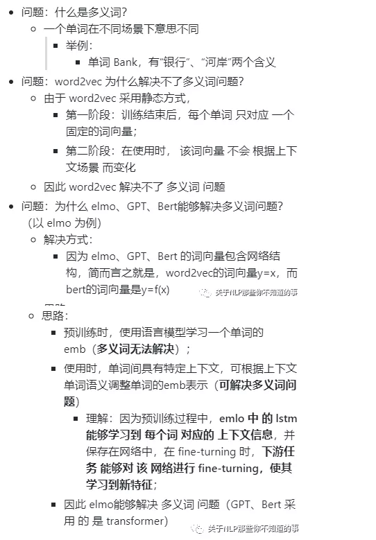
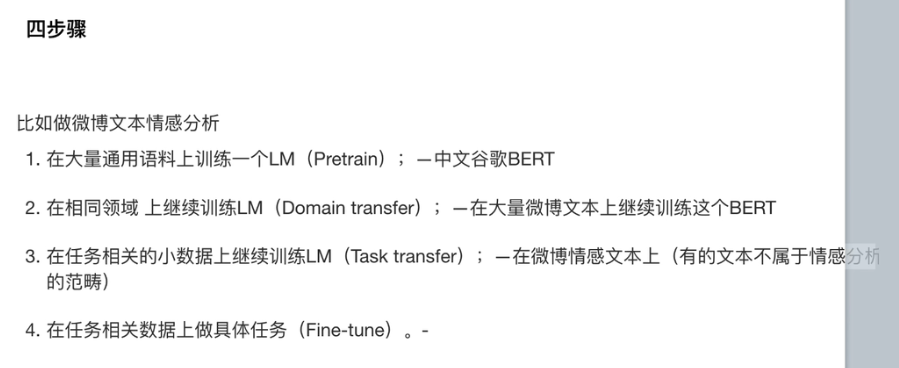
如何提高在下游任务的表现?
正常下有任务的两个步骤改为四个步骤
下面微博文本分类的例子
为什么进行softmax之前需要除 √dk
论文解释:向量的点积会很大,会将softmax函数push到梯度很小的区域,通过除会缓解这种现象
为什么是根号下dk
假设向量Q和K的各个向量q,k是互联独立的随机向量,均值为0,方差为1,那么Q点乘K的均值是0,方差是根号下dk。
为什么BERT在第一句前会加一个[CLS]标志作为整句话的语义表示,从而用于下游的分类任务等?
因为与文本中已有的其它词相比,这个无明显语义信息的符号会更“公平”地融合文本中各个词的语义信息,从而更好的表示整句话的语义。
具体来说,self-attention是用文本中的其它词来增强目标词的语义表示,但是目标词本身的语义还是会占主要部分的,因此,经过BERT的12层,每次词的embedding融合了所有词的信息,可以去更好的表示自己的语义。
而[CLS]位本身没有语义,经过12层,得到的是attention后所有词的加权平均,相比其他正常词,可以更好的表征句子语义。
Albert的改进
参数缩减方法
本文提出两种模型参数缩减的方法,具体如下:
- 从模型角度来讲,wordPiece embedding是学习上下文独立的表征维度为E,而隐藏层embedding是学习上下文相关的表征维度为H。为了应用的方便,原始的bert的向量维度E=H,这样一旦增加了H,E也就增大了。ALBert提出向量参数分解法,将一个非常大的词汇向量矩阵分解为两个小矩阵,例如词汇量大小是V,向量维度是E,隐藏层向量为H,则原始词汇向量参数大小为V * H,ALBert想将原始embedding映射到V * E(低纬度的向量),然后映射到隐藏空间H,这样参数量从 V*H下降到V * E+E * H,参数量大大下降。但是要注意这样做的损失确保矩阵分解后的两个小矩阵的乘积损失,是一个有损的操作。
- 层之间参数共享。base的bert总共由12层的transformer的encoder部分组成,层参数共享方法避免了随着深度的加深带来的参数量的增大。具体的共享参数有这几种,attention参数共享、ffn残差网络参数共享
SOP预训练任务
我们知道原始的Bert预训练的loss由两个任务组成,maskLM和NSP(Next Sentence Prediction),maskLM通过预测mask掉的词语来实现真正的双向transformer,NSP类似于语义匹配的任务,预测句子A和句子B是否匹配,是一个二分类的任务,其中正样本从原始语料获得,负样本随机负采样。NSP任务可以提高下游任务的性能,比如句子对的关系预测。但是也有论文指出NSP任务其实可以去掉,反而可以提高性能,比如RoBert。
本文以为NSP任务相对于MLM任务太简单了,学习到的东西也有限,因此本文提出了一个新的loss,sentence-order prediction(SOP),SOP关注于句子间的连贯性,而非句子间的匹配性。SOP正样本也是从原始语料中获得,负样本是原始语料的句子A和句子B交换顺序。举个例子说明NSP和SOP的区别,原始语料句子 A和B, NSP任务正样本是 AB,负样本是AC;SOP任务正样本是AB,负样本是BA。可以看出SOP任务更加难,学习到的东西更多了(句子内部排序)。
bert输入大于512的解决办法
Clipping(截断法)
对长输入进行截断,挑选其中「重要」的token输入模型。一种最常见的办法是挑选文章的前 Top N 个 token,和文末的 Top K 个 token,保证 N + K <= 510,这种方法基于的前提假设是「文章的首尾信息最能代表篇章的全局概要」;此外,还有一种 two stage 的方法:先将文章过一遍 summarize 的模型,再将 summarize 模型的输出喂给分类模型。但无论哪种截断方式,都必将会丢失一部分的文本信息,可能会导致分类错误。
Pooling(池化法)
截断法最大的问题在于需要丢掉一部分文本信息,如果我们能够保留文本中的所有信息,想办法让模型能够接收文本中的全部信息,这样就能避免文本丢失带来的影响。
句子分片
由于 BERT 最多只能接受 510 个token 的输入,因此我们需要将长文本切割成若干段。假设我们有 2 句 1000 个 token 的句子,那么我就需要先将这 2 个句子切成 4 段(第 1 个句子的 2 段 + 第 2 个句子的 2 段),并放到一个 batch 的输入中喂给模型
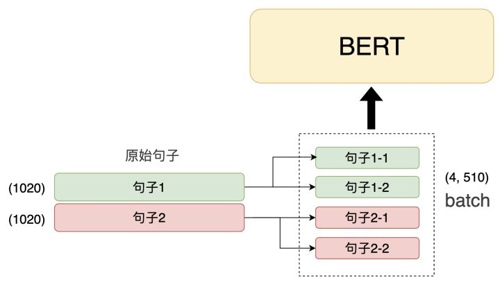
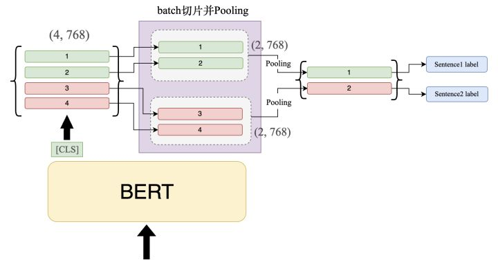
Pooling
当切完片后的数据喂给 BERT 后,我们取 BERT 模型的 [CLS] 的输出,此时输出维度应该为:(4, 768) 。随即,我们需要将这 4 个 output 按照所属句子分组,由下图所示,前 2 个向量属于一个句子,因此我们将它们归为一组,此时的维度变化:(4, 768) -> (2, 2, 768)。接着,我们对同一组的向量进行 Pooling 操作,使其下采样为 1 维的向量,即(1, 768)。Pooling 的方式有两种:Max-Pooling 和 Avg-Pooling,我们会在后面的实验中比较两种不同 Pooling 的效果。这里推荐大家使用Max-Pooling比较好,因为 Avg-Pooling 很有可能把特征值给拉平,选择保留显著特征(Max-Pooling)效果会更好一些。


 2957
2957

 被折叠的 条评论
为什么被折叠?
被折叠的 条评论
为什么被折叠?
 到【灌水乐园】发言


