动手学深度学习Task01

第一课 线性回归模型

模型简述

以预测房价为例，影响房价的只有两个因素：面积（平方米）以及房龄（年）。这里影响房价的因素称为特征（feature），真实的房价称为标签（label）。假设房价与特征之间呈线性相关，我们就可以构建一个线性回归模型如下：
$$\text{price}={\omega }_{area}\cdot x_{area}+{\omega }_{age}\cdot x_{age}+b$$
${\omega }_{area}$和${\omega }_{age}$绝对值的大小表明了面积以及房龄对房价的影响程度，$b$修正偏差。 ${\omega }_{area},{\omega }_{age}$以及$b$都是待训练优化的参数。

数据集

用于训练模型的所有样本全体称为训练集（traning set）,在本例中，一栋房子就是一个样本（sample），包含两个特征：面积以及房龄，已知真实房价。

损失函数

损失函数也是模型训练的目标函数，通常衡量的是真实值与模型预测值之间的偏差。偏差越小，说明模型预测的结果越好。本例损失函数可写为均方误差形式：
$$L(\text{w},b)=\frac{1}{n}\sum _{i=1}^n\frac{1}{2}({\text{w}}^T{\text{x}}^{(i)}+b-y^{(i)})$$
我们的目标就是最小化损失函数。

优化函数-随机梯度下降法

这里的优化函数其实就是指更新（本例就是$\text{w}$和$b$）参数的方法。我们初始化的模型参数必然会使得预测值与真实值相差很大（即上述的损失函数值很大），这时，就需要更新参数来使得损失函数值变小。本例采用的随机梯度下降法，它的思想就是函数沿着负梯度方向下降最快。具体实现：先随机初始化模型参数，接下来对参数进行多次迭代。每次迭代过程中，随机均匀采样一个固定数目的训练样本组成小批量（mini-batch）$\mathcal{B}$，然后求小批量样本数据的平均损失对模型参数的导数（梯度），沿负梯度方向下降，即模型参数直接减去梯度值即可，但通常会在梯度前乘以一个[0,1]之间的数，为下降步长，又称学习率（learning rate）。
$$(\text{w},b)\leftarrow (\text{w},b)-\frac{\eta }{|\mathcal{B}|}\sum _{i\in \mathcal{B}}{\partial }_{(\text{w},b)}{l}^{(i)}(\text{w},b)$$

线性回归的代码实现

代码实现会采用两种方法，一种从零实现，一种利用torch线性模块实现。我们首先比较矢量计算用for循坏实现以及直接矢量相加实现，其运行速度的快慢有何不同。（虽然我们早就心知肚明）

import torch
import time

n = 1000
a = torch.ones(n)
b = torch.ones(n)

# define a timer class to record time
class Timer(object):
    def __init__(self):
        self.times = []
        self.start()

    def start(self):
        # start the timer
        self.start_time = time.time()
    def stop(self):
        # stop the timer and record time into a list
        self.times.append(time.time() - self.start_time)
        return self.times[-1]
    def avg(self):
        # calculate the average and return
        return sum(self.times)/len(self.times)
    def sum(self):
        # return the sum of recorded time
        return sum(self.times)

# for循环
timer = Timer()
c = torch.zeros(n)
for i in range(n):
    c[i] = a[i] + b[i]
print('%.5f sec' % timer.stop())

# 矢量相加
timer.start()
c = a + b
print('%.5f sec' % timer.stop())

输出：
0.01325 sec
0.00000 sec

time.time()函数返回的是从1970-01-01 00:00:00起到当前时间，按秒计算，输出为过去多少秒。后者比前者快。

线性回归从零开始实现

import torch
from IPython import display
from matplotlib import pyplot as plt
import numpy as np
import random

# 生成数据集
# set input feature number
num_inputs = 2
# set examples number
num_example = 1000
#set ture weight and bias in order to generate corresponded label
true_w = [2,-3.4]
true_b = 4.2

features = torch.randn(num_example,num_inputs,dtype=torch.float32)
labels = true_w[0] * features[:,0] + true_w[1] * features[:,1] + true_b
# 由于真实标签与模型预测值是存在偏差的，因此这了添加了正态分布项来模拟真实值
labels += torch.tensor(np.random.normal(0,0.01,size=labels.size()),
                       dtype=torch.float32)

plt.scatter(features[:,1].numpy(),labels.numpy(),1)
plt.show()

# 读取数据集
def data_iter(batch_size,features,labels):
    num_example = len(features)
    indices = list(range(num_example))
    random.shuffle(indices) # 将样本排序打乱
    for i in range(0,num_example,batch_size):
        j = torch.LongTensor(indices[i:min(i+batch_size,num_example)])
        yield features.index_select(0,j), labels.index_select(0,j)

batch_size = 10

for X,y in data_iter(batch_size,features,labels):
    print(X,'\n',y)
    break

# 初始化模型参数
w = torch.tensor(np.random.normal(0,0.01,(num_inputs,1)),dtype=torch.float32)
b = torch.zeros(1,dtype=torch.float32)
# w和b是需要反向传播的
w.requires_grad_(requires_grad=True)
b.requires_grad_(requires_grad=True)

# 定义模型
def linreg(X,w,b):
    return torch.mm(X,w) + b

# 定义损失函数
def squared_loss(y_hat,y):
    # y.view是将y重新view成y_hat的size
    return (y_hat - y.view(y_hat.size())) ** 2 / 2

# 定义优化函数
def sgd(params,lr,batch_size):
    for param in params:
        # ues .data to operate param without gradient track
        param.data -= lr * param.grad / batch_size

# 训练
lr = 0.03
num_epochs = 5
net = linreg
loss = squared_loss

# traning
for epoch in range(num_epochs):
    '''
    training repeats num_epochs times
    in each epoch, all the samples in dataset will be used once
    X is the feature and y is the label of a batch sample
    '''
    for X,y in data_iter(batch_size,features,labels):
        l = loss(net(X,w,b),y).sum()
        # calculate the gradient of batch sample loss
        l.backward()
        # using small batch random gradient descent to iter model parameter
        sgd([w,b],lr,batch_size)
        #print(w,b)
        # reset parameter gradient, avoid stacking
        w.grad.data.zero_()
        b.grad.data.zero_()
        #print(w,b)
    train_l = loss(net(features,w,b),labels)
    print('epoch %d, loss %f' % (epoch+1,train_l.mean().item()))

print(w,true_w,b,true_b)

1. numpy.random.normal(loc,scale,size)正态分布:
   loc：float or array_like of floats，意义为概率分布的均值，对应分布中心；
   scale：float or array_like of floats，意义为概率分布的标准差，对应于分布的宽度，scale越大越矮胖，scale越小，越瘦高。
   size：int or tuple of ints, optional，表示输出的shape，默认为None，只输出一个值
   标准的正态分布：numpy.random.normal(loc=0.0, scale=1.0, size=None)
2. torch.tensor是32-bit floating point，torch.LongTensor是64-bit integer (signed)。
3. python中的yield函数，斐波那契数列

def fab(max):
    n, a, b = 0, 0, 1
    while n < max:
        yield b  
        a, b = b, a + b
        n = n + 1
for n in fab(5):
    print(n)

简单地讲，yield 的作用就是把一个函数变成一个 generator，带有 yield 的函数不再是一个普通函数，Python 解释器会将其视为一个 generator，调用 fab(5) 不会执行 fab 函数，而是返回一个 iterable 对象！在 for 循环执行时，每次循环都会执行 fab 函数内部的代码，执行到 yield b 时，fab 函数就返回一个迭代值，下次迭代时，代码从 yield b 的下一条语句继续执行，而函数的本地变量看起来和上次中断执行前是完全一样的，于是函数继续执行，直到再次遇到 yield。（摘自菜鸟教程，https://blog.youkuaiyun.com/mieleizhi0522/article/details/82142856这篇博客也讲得很好）

4. index_select(self,input,dim,index)：dim表示选择的维度（比如按列选择还是按行选择），index表示根据选择的维度所挑选的数据下标

import torch

a = torch.linspace(1,16,steps=16).view(4,4)
print(a,a.shape)
# 挑选的数据下标
ind = torch.tensor([0,2])
# 0表示按行索引，1表示按列索引
b = torch.index_select(a,0,ind)
print(b)
# 第二种写法
c = a.index_select(0,ind)
print(c)
输出：
tensor([[ 1.,  2.,  3.,  4.],
        [ 5.,  6.,  7.,  8.],
        [ 9., 10., 11., 12.],
        [13., 14., 15., 16.]]) torch.Size([4, 4])
tensor([[ 5.,  6.,  7.,  8.],
        [13., 14., 15., 16.]])
tensor([[ 5.,  6.,  7.,  8.],
        [13., 14., 15., 16.]])

5. view函数，神经网络代码中还常见x.view(x.size()[0],-1)，x.size()[0]通常表示batch_size，-1表示自适应(有这种情况，但不唯一)。
6. 在pytorch里面，x.item()返回的是张量x里面的元素，而不是张量x。

import torch

x = torch.tensor([1])
y = x.item()
print(x,x.type())
print(y)

output:
tensor([1]) torch.LongTensor
1

线性回归模型的PyTorch实现

import torch
from torch import nn
import numpy as np
import torch.utils.data as Data
from torch.nn import init
import torch.optim as optim
torch.manual_seed(1)

torch.set_default_tensor_type('torch.FloatTensor')

# 生成数据集
num_inputs = 2
num_examples = 1000

true_w = [2,-3.4]
true_b = 4.2
features = torch.tensor(np.random.normal(0,1,(num_examples,num_inputs)),dtype=torch.float32)
labels = true_w[0] * features[:,0] + true_w[1] * features[:,1] + true_b
labels += torch.tensor(np.random.normal(0,0.01,size=labels.size()),dtype=torch.float32)

# 读取数据集
batch_size = 10
# combine features and labels of dataset
dataset = Data.TensorDataset(features,labels)
# put dataset into DataLoader
data_iter = Data.DataLoader(
    dataset=dataset,         # torch TensorDataset format
    batch_size=batch_size,   # mini batch size
    shuffle=True,            # whether shuffle the data or not
    #num_workers=2,           # read data in multithreading
)

for X,y in data_iter:
    print(X,'\n',y)
    break

# 定义模型
class LinearNet(nn.Module):
    def __init__(self,n_feature):
        super(LinearNet,self).__init__()  # call father function to init
        self.linear = nn.Linear(n_feature,1)  # function prototype:'torch.nn.Linear(in_features,out_features,bias=True)'

    def forward(self,x):
        y = self.linear(x)
        return y
net = LinearNet(num_inputs)
print(net)

net = nn.Sequential(
    nn.Linear(num_inputs,1)
)
# 初始化参数模型
init.normal_(net[0].weight,mean=0.0,std=0.01)
init.constant_(net[0].bias,val=0.0)  # or you can use 'net[0].bias.data.fill_(0)' to modify it directly

for param in net.parameters():
    print(param)

# 定义损失函数
loss = nn.MSELoss() # nn built-in squared loss function
                    # function prototype: `torch.nn.MSELoss(size_average=None, reduce=None, reduction='mean')`

# 定义优化函数
optimizer = optim.SGD(net.parameters(),lr=0.03)
print(optimizer)

# 训练
num_epochs = 3
for epoch in range(1,num_epochs+1):
    for X,y in data_iter:
        output = net(X)
        l = loss(output,y.view(-1,1))
        optimizer.zero_grad()
        l.backward()
        optimizer.step()
    print('epoch %d, loss: %f' % (epoch,l.item()))

dense = net[0]
print(true_w, dense.weight.data)
print(true_b,dense.bias.data)

构建多层网络的三种方法

from torch import nn

# method 1
net = nn.Sequential(
    nn.Linear(num_inputs,1)
    # other layers can be added here
)

# method 2
net = nn.Sequential()
net.add_module('Linear',nn.Linear(num_inputs,1))
# net.add_module ......

# method 3
from collections import OrderedDict
net = nn.Sequential(OrderedDict([
          ('linear', nn.Linear(num_inputs, 1))
          # ......
        ]))

1. torch.manual_seed(1)：随机初始化种子，保证每次初始化的值相同

第二课 softmax和分类模型

softmax的基本概念

关于softmax的基本概念，课程中讲解的十分详细，且优快云上也有诸多相关文章，这里就不赘述。仅记下重要公式。

softmax回归模型

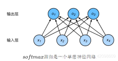
$$o_1=x_1{\omega }_{11}+x_2{\omega }_{21}+x_3{\omega }_{31}+x_4{\omega }_{41}+b_1$$

$$o_2=x_1{\omega }_{12}+x_2{\omega }_{22}+x_3{\omega }_{32}+x_4{\omega }_{42}+b_2$$

$$o_3=x_1{\omega }_{13}+x_2{\omega }_{23}+x_3{\omega }_{33}+x_4{\omega }_{43}+b_3$$
$x_i$表示第$i$个特征，$o_i$表示是第$i$类的得分，得分越高，为第$i$类的可能性就越大。
由于直接输出后存在两个问题：

1. 一方面，由于输出层的输出值的范围不确定，我们难以直观上判断这些值的意义。
2. 另一方面，由于真实标签是离散值，这些离散值与不确定范围的输出值之间的误差难以衡量。

因此采用softmax运算将输出归一化到[0,1]之间，解决了这一问题。softmax运算具体表示：
$${\hat{y}}^i=\frac{\exp (o_i)}{{\sum }_{j=1}^3{\exp }_{(o_j)}}，\sum _i{\hat{y}}^i=1$$
因此，softmax回归模型（对单个样本）可简写为：
$$o^{(i)}=x^{(i)}W+b$$

$${\hat{y}}^{(i)}=softmax(o^{(i)})$$
对应代码

def softmax(X):
    X_exp = X.exp()
    partition = X_exp.sum(dim=1, keepdim=True)
    # print("X size is ", X_exp.size())
    # print("partition size is ", partition, partition.size())
    return X_exp / partition  # 这里应用了广播机制

交叉熵损失函数

不采用平方损失函数，因为在这种多分类情况下，每个样本针对每个标签都有一个得分，但真实标签只是其中一个，平方损失函数的值会随着非标签的预测值浮动。
交叉熵（对单个样本）
$$H(y^{(i)},{\hat{y}}^{(i)})=-\sum _{j=1}^q{y}_j^{(i)}\log {\hat{y}}_j^{(i)}$$

因为$y^{(i)}$里面的元素非0即1，假设$y_k^{(i)}$为1，其余为0，则等式可以重新写为
$$H(y^{(i)},{\hat{y}}^{(i)})=-\log {\hat{y}}_k^{(i)}$$

从这个等式就可以看出，交叉熵只考虑预测值最高的样本，预测值越大，交叉熵的值越小。
假设训练数据样本为$n$，交叉熵损失函数定义为
$$l(\Theta )=\frac{1}{n}\sum _{i=1}^{n}H(y^{(i)},{\hat{y}}^{(i)})$$

对应代码

def cross_entropy(y_hat, y):
    return - torch.log(y_hat.gather(1, y.view(-1, 1)))

在这里顺便记一下gether函数的用法：gather(dim,index)，它是取值操作，dim表示按行取还是按列取，0表示按列取，1表示按行取。index表示取值的下标。

y_hat = torch.tensor([[0.1, 0.3, 0.6], [0.3, 0.2, 0.5]])
y = torch.LongTensor([0, 2])
y_hat.gather(1, y.view(-1, 1))
output:
tensor([[0.1000],
        [0.5000]])

这里必须为y.view(-1, 1)，如果改成y.view(1, -1)会报错。

对多维Tensor按维度操作

X = torch.tensor([[1, 2, 3], [4, 5, 6]])
print(X.sum(dim=0, keepdim=True))  # dim为0，按照相同的列求和，并在结果中保留列特征
print(X.sum(dim=1, keepdim=True))  # dim为1，按照相同的行求和，并在结果中保留行特征
print(X.sum(dim=0, keepdim=False)) # dim为0，按照相同的列求和，不在结果中保留列特征
print(X.sum(dim=1, keepdim=False)) # dim为1，按照相同的行求和，不在结果中保留行特征
output:
tensor([[5, 7, 9]])
tensor([[ 6],
        [15]])
tensor([5, 7, 9])
tensor([ 6, 15])

其他函数

1. iter()函数：生成了一个迭代器。

list_ = [1, 2, 3, 4, 5]
it = iter(list_)
for i in range(5):
    line = next(it)
    print("第%d 行， %s" %(i, line))
output:
第0 行， 1
第1 行， 2
第2 行， 3
第3 行， 4
第4 行， 5

第三课 多层感知机

多层感知机的基本介绍

课程讲解的十分详尽，这里就简记一下知识点。
下图展示了一个多层感知机的神经网络图，它含有一个隐藏层，该层中有5个隐藏单元。

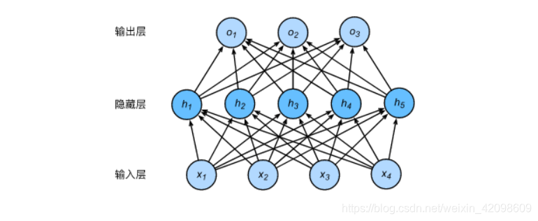
含单隐藏层的多层感知机，其输出$O^{n\times q}$计算为（$n$是批量大小，$q$是输出类别数）：
$$H=X{W}_h+b_h$$

$$O=H{W}_o+b_o$$

联立起来得
$$O=(X{W}_h+b_h)W_o+b_o=X{W}_h{W}_o+b_h{W}_o+b_o$$

不难看出，输出与输入特征仍为线性关系，事实上，即便再添加更多的隐藏层，以上设计依然只能与仅含输出层的单层神经网络等价。

激活函数

激活函数引入了非线性变换。
这里有三种激活函数：relu函数、sigmoid函数以及tanh函数。
relu函数：
$$ReLU(x)=max(x,0)$$

sigmoid函数：
$$sigmoid(x)=\frac{1}{1+\exp (-x)}$$

由此可见，sigmoid函数取值在[0,1]之间。
sigmoid导数：
$$sigmoi{d}^{\prime }(x)=sigmoid(x)(1-sigmoid(x))$$

tanh函数：
$$tanh(x)=\frac{1-\exp (-2x)}{1+\exp (-2x)}=\frac{2}{1+\exp (-2x)}-1$$

由此可见，tanh函数取值在[-1,1]之间。
tanh函数导数：
$$tan{h}^{\prime }(x)=1-tan{h}^2(x)$$

它是关于原点对称的。

关于激活函数的选择

ReLu函数是一个通用的激活函数，目前在大多数情况下使用。但是，ReLU函数只能在隐藏层中使用。

用于分类器时，sigmoid函数及其组合通常效果更好。由于梯度消失问题，有时要避免使用sigmoid和tanh函数（因为它们的梯度在[0,1]之间）。

在神经网络层数较多的时候，最好使用ReLu函数，ReLu函数比较简单计算量少，而sigmoid和tanh函数计算量大很多。

在选择激活函数的时候可以先选用ReLu函数如果效果不理想可以尝试其他激活函数。

多层感知机代码解读

多层感知机就是含有至少一个隐藏层的由全连接层组成的神经网络，且每个隐藏层的输出通过激活函数进行变换。
$$H=\Phi (X{W}_h+b_h)$$

$$O=H{W}_o+b_o$$

从零开始实现需自己定义网络

def net(X):
    X = X.view((-1, num_inputs))
    #隐藏层输出
    H = relu(torch.matmul(X, W1) + b1)
    return torch.matmul(H, W2) + b2

torch.matmul(tensor1,tensor2,out=None)
torch.mm(mat1,mat2,out=None)
二者之间的区别从输入参数上就可以看出。

利用PyTorch实现时

net = nn.Sequential(
        # FlattenLayer是在数据输入前进行维度变换
        d2l.FlattenLayer(),
        nn.Linear(num_inputs, num_hiddens),
        nn.ReLU(),
        nn.Linear(num_hiddens, num_outputs), 
        )

其他函数

1. detch()函数：简而言之就是将参数从网络中隔离开来，不再参与更新。一个简单的示例摘自慢行厚积：

import torch

a = torch.tensor([1, 2, 3.], requires_grad=True)
print(a.grad)
out = a.sigmoid()
print(out)

#添加detach(),c的requires_grad为False
c = out.detach()
print(c)

#这时候没有对c进行更改，所以并不会影响backward()
out.sum().backward()
print(a.grad)
output:
None
tensor([0.7311, 0.8808, 0.9526], grad_fn=<SigmoidBackward>)
tensor([0.7311, 0.8808, 0.9526])
tensor([0.1966, 0.1050, 0.0452])