量子计算 16 量子算法1

之前了解到因为量子电路难以确定，以及其硬件设备目前还处于很初步的发展阶段，我们通常就会用查询复杂度(Query Complexity)来讨论量子算法。

尽管硬件还没有成熟，但我们已经在查询复杂度的基础上分析发展了一些厉害的量子算法了，今天来介绍第一部分。

1 The Deutsch-Jozsa Algorithm

Problem: f : { 0 , 1 } n → { 0 , 1 } f: \{0,1\}^n\rightarrow\{0,1\} f:{0,1}n→{0,1}, Compute $f(0)\oplus f(1)$, namely XOR.

• 经典算法中，不管是确定性算法还是随机算法，显然需要调用两次函数$f$才能解决该问题。
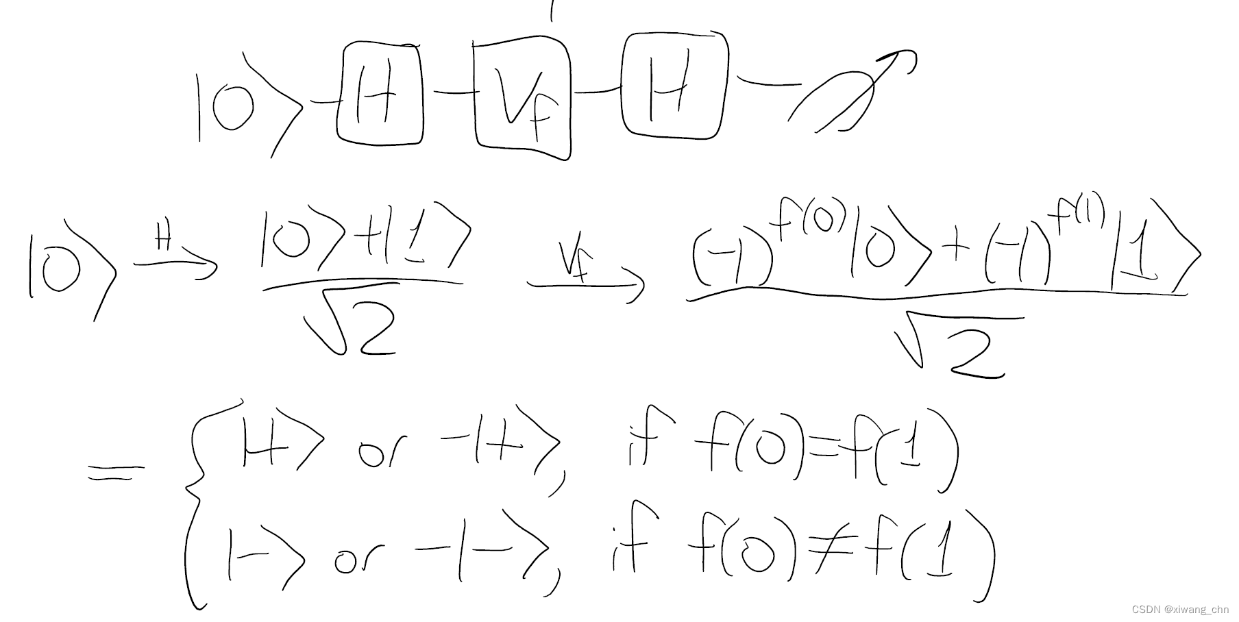
• 量子算法中，仅需要调用一次函数就可以解决该问题。如下图所示，经过Hadamard门、phase query和Hadamard门操作后，在基$|+⟩,|-⟩$下测量，即可得$f(0)\oplus f(1)$，回顾下XOR操作是相异为1。
  

Generalization 1: Compute the parity of N bits, $f(0)\oplus f(1)\cdots \oplus f(N-1)$

这个很简答，就重复用原来的算法即可，这样的话量子查询复杂度就是$Q(\text{Parity})=\lceil N/2\rceil$，经典查询复杂度$D(\text{Parity})=R(\text{Parity})=N$。

$D$代表经典确定算法查询复杂度；$R$代表经典随机算法查询复杂度；$Q$代表量子算法查询复杂度；

Generalization 2: f : { 0 , 1 } n → { 0 , 1 } f: \{0,1\}^n\rightarrow\{0,1\} f:{0,1}n→{0,1}, decide $f$ is constant or balanced (equal # of 0 or 1)

$D=\Omega (2^n),R=O(1),Q=1$
证明过程私信

2 The Bernstein-Vazirani Algorithm

Problem: Given f : { 0 , 1 } n → { 0 , 1 } f: \{0,1\}^n\rightarrow\{0,1\} f:{0,1}n→{0,1}. Promised that ∃ s ∈ { 0 , 1 } n \exists s\in \{0,1\}^n ∃s∈{0,1}n, s.t. $\forall x,f(x)=s\cdot x(\text{mod}2)$. Find the secret string $s$

经典查询复杂度 $D=R=n$

显然，每次查询，如x=100, 010, 001，都只能得到$s$的第一、二、三个bit的值。

量子查询复杂度$Q=1$, beyond exponential speedup

先回顾我们的老朋友Hadamard门，如下图，H门其实是改变了量子比特的phase，且是可逆的，再次施加H门又会恢复原样；

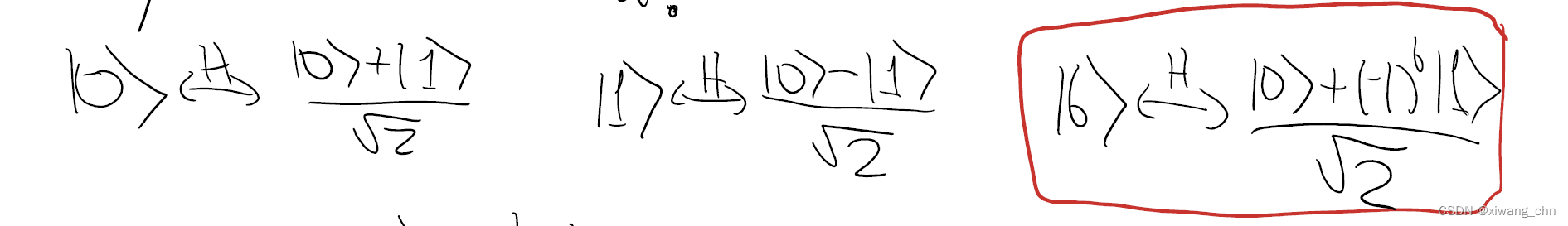
如果对多个qubit同时施加Hadamard门，如下图，首先将系数提出，则量子幅的正负就是由$|1⟩$的系数决定。

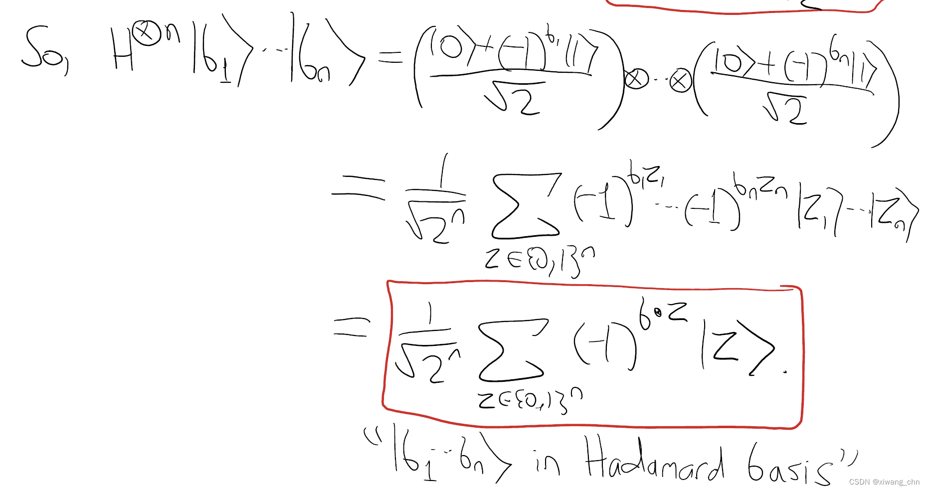
则量子算法如下图所示，这也代表了量子算法的经典结构，先创建一些叠加态，查询之后再转换一下叠加态最后测量。

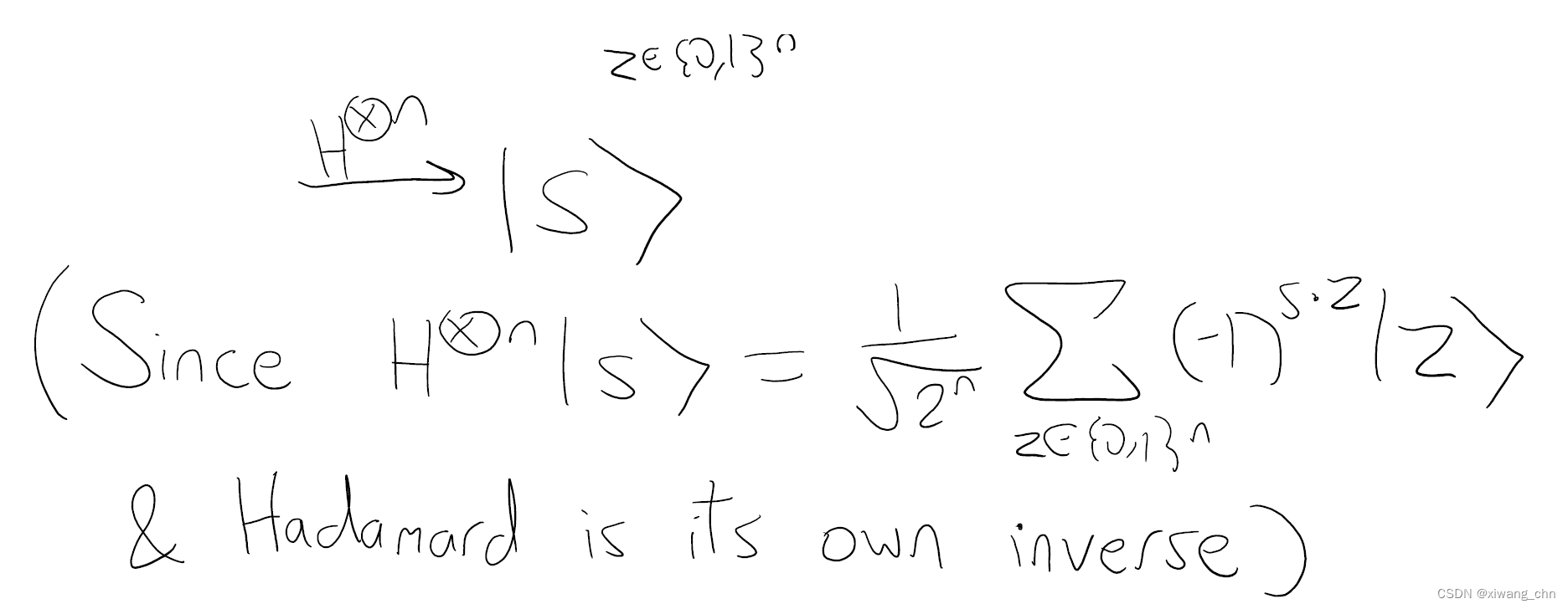
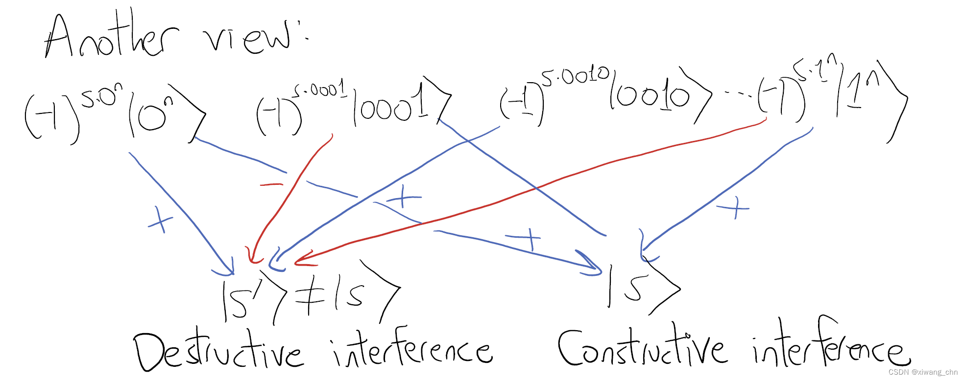
如我们在 量子计算 12 中所说的那样，其实量子算法的过程是通过调整量子干涉，使得一些结果的量子幅为零，另一些的量子幅变大，从而使得测量结果是我们想要的结果，如下图，查询后的量子比特，经过H门后将想要的结果量子幅变大，而其他的量子幅抵消掉。

这里虽然仅进行了一次查询，但是做了$n$次测量，因此得到了$n$个bit的信息。而1与$n$的复杂度，也是相当大，因为我们一半认为从$n$到$\log n$就是指数加速了，而本算法可以首先超指数的加速。

3 Simon’s Problem and Its Classical Query Complexity

虽然BV(Bernstein-Vazirani)算法的加速很大，但是这个问题并不难，经典算法的复杂度也就是$O(n)$而已。因此我们来看个经典复杂度较大的问题，Simon’s Problem.

Simon’s Problem: Given f : { 0 , 1 } n → { 0 , 1 } n f: \{0,1\}^n\rightarrow\{0,1\}^n f:{0,1}n→{0,1}n. Promised that ∃ s ≠ 0 n ∈ { 0 , 1 } n \exists s\ne0^n \in \{0,1\}^n ∃s​=0n∈{0,1}n, s.t. $\forall x\ne y,f(x)=f(y)⟺y=x\oplus s$. Find $s$.

Decision variant: Promised that $f$ either satisfies Simon (2 to 1) promise or is 1 to 1.

如果满足Simon’s promise, 说明对于任意input x, string s 将它们分成了两类，根据s的1的位，将对应的x的位翻转，所对应的$f(x)$不变，这是异或XOR的性质，而翻转与否则正好是数量相等的两类，说明这个函数$f(x)$是2 to 1的map，即两个输入map到一个输出上面。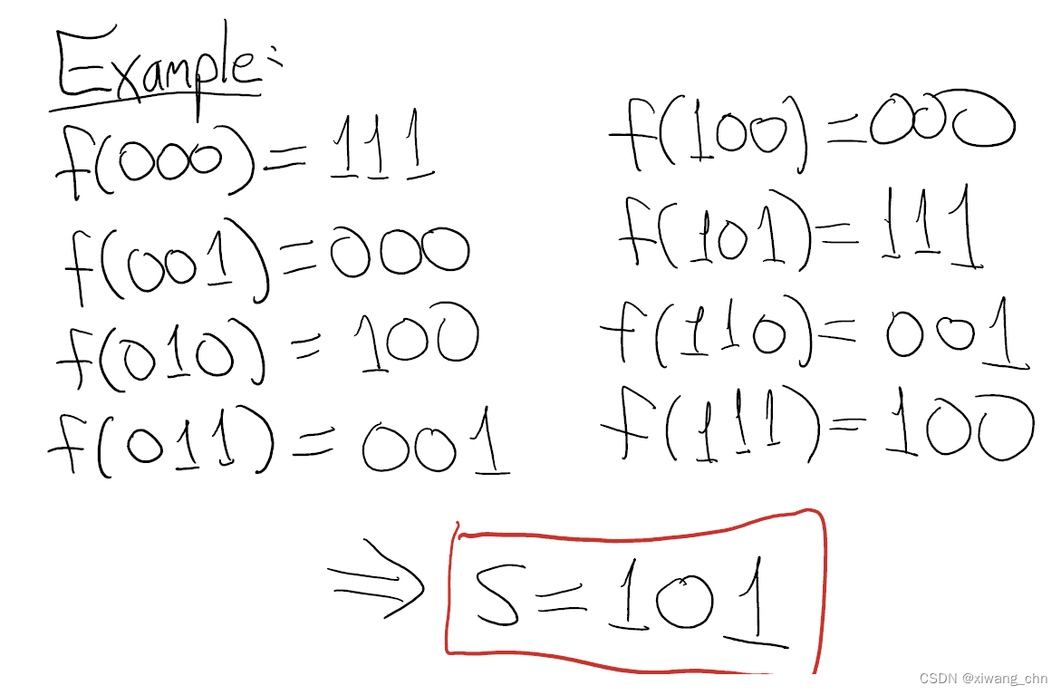

经典查询复杂度

这里要用到随机算法，即随机选定一些输入，来看其能出现$f(x)=f(y)$的概率，如果出现了说明$x=y\oplus s⟺s=x\oplus y$

Birthday Paradox

简单来说，如果23个人在同一个房间里，那么50%的概率有两个人的生日是同一天。也是简单的概率问题，$1-\frac{A_N^T}{N^T}$wiki，即$\approx 1-(1-365\times \frac{1}{365}\times \frac{1}{365}{)}^{\left(\genfrac{}{}{0ex}{}{23}{2}\right)}\approx 0.5$，即$1-(1-\epsilon {)}^n=\Theta (n\epsilon )=\Theta (\left(\genfrac{}{}{0ex}{}{T}{2}\right)\epsilon )=\Theta (\left(\genfrac{}{}{0ex}{}{T}{2}\right)\frac{1}{N})=1$，则要让T个人在N天一年的生日一致的概率很高的话，则需要$T=\Theta (N^{1/2})$个人。

Proof

同样的，在Simon算法中，共有$2^{n-1}$个不同的输出，也就是$2^{n-1}$天，那我需要挑$\Theta (N^{1/2})$个输入，则有两个输入是同一天，也就是同一个输出的概率才比较大，因此Simon经典算法的复杂度为$\Theta (N^{1/2})$。

这也是经典算法最好的结果。

假设，任意一个确定算法选取了T个输入$x_1,\dots ,x_T$，根据Union bound:
$\mathrm{Pr}(\text{Collision})\le {\sum }_{1\le i<j\le T}\mathrm{Pr}[f(x_i)=f(x_j)]={\sum }_{1\le i<j\le T}\frac{2^{n-1}}{\left(\genfrac{}{}{0ex}{}{2^n}{2}\right)}={\sum }_{1\le i<j\le T}\frac{1}{2^n-1}=\frac{\left(\genfrac{}{}{0ex}{}{T}{2}\right)}{2^n-1}$

如果$T=O(2^{n/2})$则概率为$O(1)$，如果小于，则还剩$2^n-1-\left(\genfrac{}{}{0ex}{}{T}{2}\right)$个$s$要排除，而任意随机算法，都相当于这些经典确定算法的凸组合，因此任意的经典算法都需要$\Omega (2^{n/2})$个查询复杂度。

量子查询复杂度-见下回分解