TensorFlow学习DAY5tensorboard网络结构

最新推荐文章于 2025-06-13 10:36:52 发布

原创最新推荐文章于 2025-06-13 10:36:52 发布 · 215 阅读

0 ·

CC 4.0 BY-SA版权

文章标签：

#tensorflow #深度学习

本文详细介绍了如何通过调整神经网络结构、优化器和迭代次数来提高MNIST数据集上的分类准确率，同时深入探讨了TensorBoard的配置与使用，包括参数概要、网络运行可视化及T-SNE训练成果展示。

摘要生成于 C知道，由 DeepSeek-R1 满血版支持，前往体验 >

首先对上一次的准确率进行提高

代码如下：

import tensorflow as tf
from tensorflow.examples.tutorials.mnist import input_data

#载入数据集
mnist = input_data.read_data_sets("MNIST_data",one_hot=True)

#每个批次的大小
batch_size = 100
#计算一共有多少个批次
n_batch = mnist.train.num_examples // batch_size

#定义两个placeholder
x = tf.placeholder(tf.float32,[None,784])
y = tf.placeholder(tf.float32,[None,10])
keep_prob=tf.placeholder(tf.float32)
lr = tf.Variable(0.001, dtype=tf.float32)

#创建一个简单的神经网络
W1 = tf.Variable(tf.truncated_normal([784,500],stddev=0.1))
b1 = tf.Variable(tf.zeros([500])+0.1)
L1 = tf.nn.tanh(tf.matmul(x,W1)+b1)
L1_drop = tf.nn.dropout(L1,keep_prob) 

W2 = tf.Variable(tf.truncated_normal([500,300],stddev=0.1))
b2 = tf.Variable(tf.zeros([300])+0.1)
L2 = tf.nn.tanh(tf.matmul(L1_drop,W2)+b2)
L2_drop = tf.nn.dropout(L2,keep_prob) 

W3 = tf.Variable(tf.truncated_normal([300,10],stddev=0.1))
b3 = tf.Variable(tf.zeros([10])+0.1)
prediction = tf.nn.softmax(tf.matmul(L2_drop,W3)+b3)

#交叉熵代价函数
loss = tf.reduce_mean(tf.nn.softmax_cross_entropy_with_logits(labels=y,logits=prediction))
#训练
train_step = tf.train.AdamOptimizer(lr).minimize(loss)

#初始化变量
init = tf.global_variables_initializer()

#结果存放在一个布尔型列表中
correct_prediction = tf.equal(tf.argmax(y,1),tf.argmax(prediction,1))#argmax返回一维张量中最大的值所在的位置
#求准确率
accuracy = tf.reduce_mean(tf.cast(correct_prediction,tf.float32))

with tf.Session() as sess:
    sess.run(init)
    for epoch in range(51):
        sess.run(tf.assign(lr, 0.001 * (0.95 ** epoch)))#使学习率逐渐减小
        for batch in range(n_batch):
            batch_xs,batch_ys =  mnist.train.next_batch(batch_size)
            sess.run(train_step,feed_dict={x:batch_xs,y:batch_ys,keep_prob:1.0})
        
        learning_rate = sess.run(lr)
        acc = sess.run(accuracy,feed_dict={x:mnist.test.images,y:mnist.test.labels,keep_prob:1.0})
        print ("Iter " + str(epoch) + ", Testing Accuracy= " + str(acc) + ", Learning Rate= " + str(learning_rate))

运行结果如下：

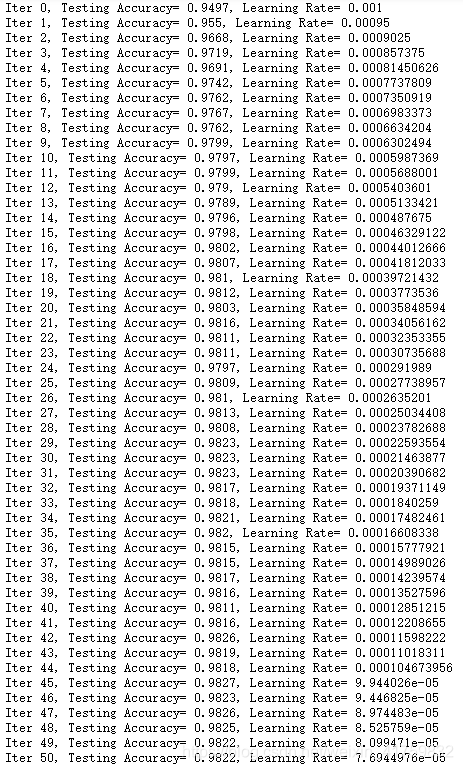
改变了中间层层数，使用Adam优化器，增加迭代次数，并且每迭代一次使得学习率减少，最终可见准确率已高达98.22%。

连接Tensorboard

代码如下

import tensorflow as tf
from tensorflow.examples.tutorials.mnist import input_data

#载入数据集
mnist = input_data.read_data_sets("MNIST_data",one_hot=True)

#每个批次的大小
batch_size = 100
#计算一共有多少个批次
n_batch = mnist.train.num_examples // batch_size

#命名空间
with tf.name_scope('input'):
    #定义两个placeholder
    x = tf.placeholder(tf.float32,[None,784],name='x-input')
    y = tf.placeholder(tf.float32,[None,10],name='y-input')

    
with tf.name_scope('layer'):
    #创建一个简单的神经网络
    with tf.name_scope('wights'):
        W = tf.Variable(tf.zeros([784,10]),name='W')
    with tf.name_scope('biases'):    
        b = tf.Variable(tf.zeros([10]),name='b')
    with tf.name_scope('wx_plus_b'):
        wx_plus_b = tf.matmul(x,W) + b
    with tf.name_scope('softmax'):
        prediction = tf.nn.softmax(wx_plus_b)

#二次代价函数
# loss = tf.reduce_mean(tf.square(y-prediction))
with tf.name_scope('loss'):
    loss = tf.reduce_mean(tf.nn.softmax_cross_entropy_with_logits(labels=y,logits=prediction))
with tf.name_scope('train'):
    #使用梯度下降法
    train_step = tf.train.GradientDescentOptimizer(0.2).minimize(loss)

#初始化变量
init = tf.global_variables_initializer()

with tf.name_scope('accuracy'):
    with tf.name_scope('correct_prediction'):
        #结果存放在一个布尔型列表中
        correct_prediction = tf.equal(tf.argmax(y,1),tf.argmax(prediction,1))#argmax返回一维张量中最大的值所在的位置
    with tf.name_scope('accuracy'):
        #求准确率
        accuracy = tf.reduce_mean(tf.cast(correct_prediction,tf.float32))

with tf.Session() as sess:
    sess.run(init)
    writer = tf.summary.FileWriter('logs/',sess.graph)
    for epoch in range(1):
        for batch in range(n_batch):
            batch_xs,batch_ys =  mnist.train.next_batch(batch_size)
            sess.run(train_step,feed_dict={x:batch_xs,y:batch_ys})
        
        acc = sess.run(accuracy,feed_dict={x:mnist.test.images,y:mnist.test.labels})
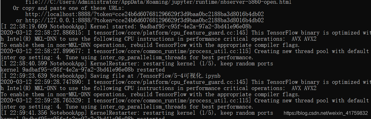
        print("Iter " + str(epoch) + ",Testing Accuracy " + str(acc))

在C盘这个地方便出现了event文件

然后按照网上方法用cmd输入tensorboard --logdir=C:\Users\Administrator\TensorFlow\logs却失败了，显示ImportError: DLL load failed: 找不到指定的模块。

查了其他博客发现一种方法

https://blog.youkuaiyun.com/qq_27855219/article/details/89449918

启动Anaconda Prompt
输入tensorboard --logdir=路径 --host=127.0.0.1

我的路径是C:\Users\Administrator\TensorFlow\logs

然后就成功了

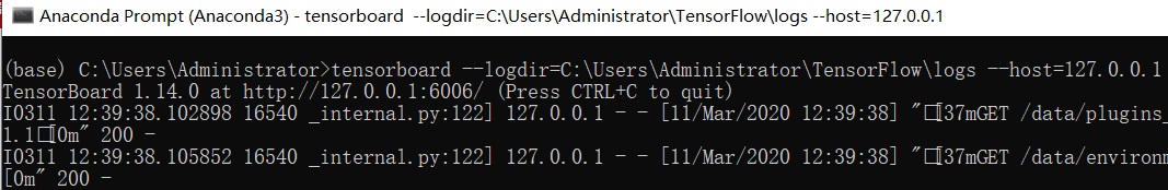
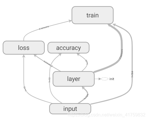
把网址复制到谷歌浏览器打开便可打开Tensorboard

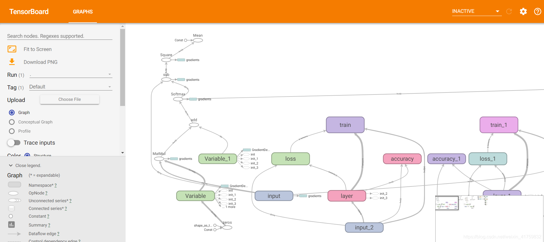
Tensorboard网络运行

相比上面的情况增加了一些参数

import tensorflow as tf
from tensorflow.examples.tutorials.mnist import input_data

#载入数据集
mnist = input_data.read_data_sets("MNIST_data",one_hot=True)

#每个批次的大小
batch_size = 100
#计算一共有多少个批次
n_batch = mnist.train.num_examples // batch_size

#参数概要
def variable_summaries(var):
    with tf.name_scope('summaries'):
        mean = tf.reduce_mean(var)
        tf.summary.scalar('mean', mean)#平均值
        with tf.name_scope('stddev'):
            stddev = tf.sqrt(tf.reduce_mean(tf.square(var - mean)))
        tf.summary.scalar('stddev', stddev)#标准差
        tf.summary.scalar('max', tf.reduce_max(var))#最大值
        tf.summary.scalar('min', tf.reduce_min(var))#最小值
        tf.summary.histogram('histogram', var)#直方图

#命名空间
with tf.name_scope('input'):
    #定义两个placeholder
    x = tf.placeholder(tf.float32,[None,784],name='x-input')
    y = tf.placeholder(tf.float32,[None,10],name='y-input')
    
with tf.name_scope('layer'):
    #创建一个简单的神经网络
    with tf.name_scope('wights'):
        W = tf.Variable(tf.zeros([784,10]),name='W')
        variable_summaries(W)
    with tf.name_scope('biases'):    
        b = tf.Variable(tf.zeros([10]),name='b')
        variable_summaries(b)
    with tf.name_scope('wx_plus_b'):
        wx_plus_b = tf.matmul(x,W) + b
    with tf.name_scope('softmax'):
        prediction = tf.nn.softmax(wx_plus_b)

#二次代价函数
# loss = tf.reduce_mean(tf.square(y-prediction))
with tf.name_scope('loss'):
    loss = tf.reduce_mean(tf.nn.softmax_cross_entropy_with_logits(labels=y,logits=prediction))
    tf.summary.scalar('loss',loss)
with tf.name_scope('train'):
    #使用梯度下降法
    train_step = tf.train.GradientDescentOptimizer(0.2).minimize(loss)

#初始化变量
init = tf.global_variables_initializer()

with tf.name_scope('accuracy'):
    with tf.name_scope('correct_prediction'):
        #结果存放在一个布尔型列表中
        correct_prediction = tf.equal(tf.argmax(y,1),tf.argmax(prediction,1))#argmax返回一维张量中最大的值所在的位置
    with tf.name_scope('accuracy'):
        #求准确率
        accuracy = tf.reduce_mean(tf.cast(correct_prediction,tf.float32))
        tf.summary.scalar('accuracy',accuracy)
        
#合并所有的summary
merged = tf.summary.merge_all()

with tf.Session() as sess:
    sess.run(init)
    writer = tf.summary.FileWriter('logs/',sess.graph)
    for epoch in range(51):
        for batch in range(n_batch):
            batch_xs,batch_ys =  mnist.train.next_batch(batch_size)
            summary,_ = sess.run([merged,train_step],feed_dict={x:batch_xs,y:batch_ys})
            
        writer.add_summary(summary,epoch)
        acc = sess.run(accuracy,feed_dict={x:mnist.test.images,y:mnist.test.labels})
        print("Iter " + str(epoch) + ",Testing Accuracy " + str(acc))

显示在Tensorboard如下

另外可显示正确率，灰色的线代表真实准确率，可调左边的smoothing使这个折线平滑

还可以看到其他曲线

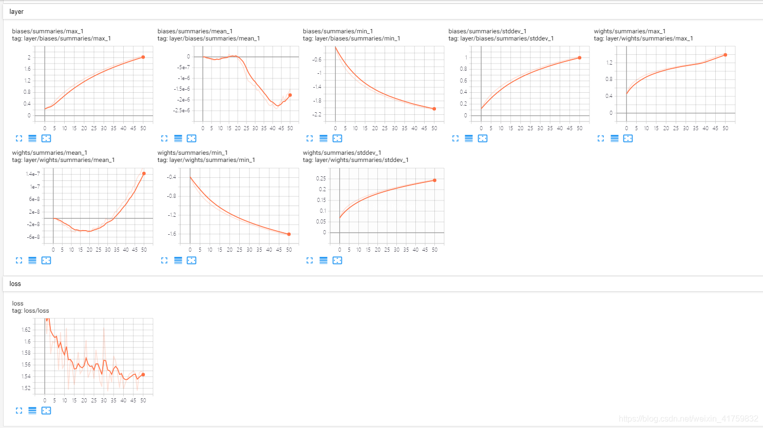
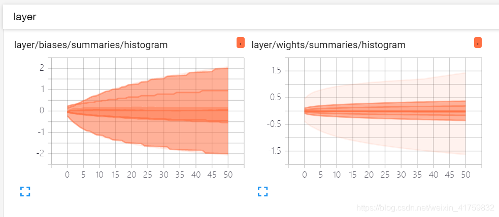
还可看到偏置值和权值的分布图，颜色越深代表分布越多

TensorBoard可视化

代码如下

import tensorflow as tf
from tensorflow.examples.tutorials.mnist import input_data
from tensorflow.contrib.tensorboard.plugins import projector


#载入数据集
mnist = input_data.read_data_sets("MNIST_data/",one_hot=True)
#运行次数
max_steps = 1001
#图片数量
image_num = 3000
#文件路径
DIR = "C:/Users/Administrator/TensorFlow/"

#定义会话
sess = tf.Session()

#载入图片
embedding = tf.Variable(tf.stack(mnist.test.images[:image_num]), trainable=False, name='embedding')

#参数概要
def variable_summaries(var):
    with tf.name_scope('summaries'):
        mean = tf.reduce_mean(var)
        tf.summary.scalar('mean', mean)#平均值
        with tf.name_scope('stddev'):
            stddev = tf.sqrt(tf.reduce_mean(tf.square(var - mean)))
        tf.summary.scalar('stddev', stddev)#标准差
        tf.summary.scalar('max', tf.reduce_max(var))#最大值
        tf.summary.scalar('min', tf.reduce_min(var))#最小值
        tf.summary.histogram('histogram', var)#直方图

#命名空间
with tf.name_scope('input'):
    #这里的none表示第一个维度可以是任意的长度
    x = tf.placeholder(tf.float32,[None,784],name='x-input')
    #正确的标签
    y = tf.placeholder(tf.float32,[None,10],name='y-input')

#显示图片
with tf.name_scope('input_reshape'):
    image_shaped_input = tf.reshape(x, [-1, 28, 28, 1])
    tf.summary.image('input', image_shaped_input, 10)

with tf.name_scope('layer'):
    #创建一个简单神经网络
    with tf.name_scope('weights'):
        W = tf.Variable(tf.zeros([784,10]),name='W')
        variable_summaries(W)
    with tf.name_scope('biases'):
        b = tf.Variable(tf.zeros([10]),name='b')
        variable_summaries(b)
    with tf.name_scope('wx_plus_b'):
        wx_plus_b = tf.matmul(x,W) + b
    with tf.name_scope('softmax'):    
        prediction = tf.nn.softmax(wx_plus_b)

with tf.name_scope('loss'):
    #交叉熵代价函数
    loss = tf.reduce_mean(tf.nn.softmax_cross_entropy_with_logits(labels=y,logits=prediction))
    tf.summary.scalar('loss',loss)
with tf.name_scope('train'):
    #使用梯度下降法
    train_step = tf.train.GradientDescentOptimizer(0.5).minimize(loss)

#初始化变量
sess.run(tf.global_variables_initializer())

with tf.name_scope('accuracy'):
    with tf.name_scope('correct_prediction'):
        #结果存放在一个布尔型列表中
        correct_prediction = tf.equal(tf.argmax(y,1),tf.argmax(prediction,1))#argmax返回一维张量中最大的值所在的位置
    with tf.name_scope('accuracy'):
        #求准确率
        accuracy = tf.reduce_mean(tf.cast(correct_prediction,tf.float32))#把correct_prediction变为float32类型
        tf.summary.scalar('accuracy',accuracy)

#产生metadata文件
if tf.gfile.Exists(DIR + 'projector/projector/metadata.tsv'):
    tf.gfile.DeleteRecursively(DIR + 'projector/projector/metadata.tsv')
with open(DIR + 'projector/projector/metadata.tsv', 'w') as f:
    labels = sess.run(tf.argmax(mnist.test.labels[:],1))
    for i in range(image_num):   
        f.write(str(labels[i]) + '\n')        
        
#合并所有的summary
merged = tf.summary.merge_all()   


projector_writer = tf.summary.FileWriter(DIR + 'projector/projector',sess.graph)
saver = tf.train.Saver()
config = projector.ProjectorConfig()
embed = config.embeddings.add()
embed.tensor_name = embedding.name
embed.metadata_path = DIR + 'projector/projector/metadata.tsv'
embed.sprite.image_path = DIR + 'projector/data/mnist_10k_sprite.png'
embed.sprite.single_image_dim.extend([28,28])
projector.visualize_embeddings(projector_writer,config)

for i in range(max_steps):
    #每个批次100个样本
    batch_xs,batch_ys = mnist.train.next_batch(100)
    run_options = tf.RunOptions(trace_level=tf.RunOptions.FULL_TRACE)
    run_metadata = tf.RunMetadata()
    summary,_ = sess.run([merged,train_step],feed_dict={x:batch_xs,y:batch_ys},options=run_options,run_metadata=run_metadata)
    projector_writer.add_run_metadata(run_metadata, 'step%03d' % i)
    projector_writer.add_summary(summary, i)
    
    if i%100 == 0:
        acc = sess.run(accuracy,feed_dict={x:mnist.test.images,y:mnist.test.labels})
        print ("Iter " + str(i) + ", Testing Accuracy= " + str(acc))

saver.save(sess, DIR + 'projector/projector/a_model.ckpt', global_step=max_steps)
projector_writer.close()
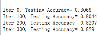
sess.close()

运行发现程序报错如下

通过上网查资料发现是因为内存不足，之后我把运行次数变为301，图片数量不变，便运行成功了。结果如下

之后再Anaconda Prompt输入tensorboard --logdir=C:\Users\Administrator\TensorFlow\projector\projector --host=127.0.0.1

打开了TensorBoard便可看到这个三维图片（感动死了~~~~(>_<)~~~~）

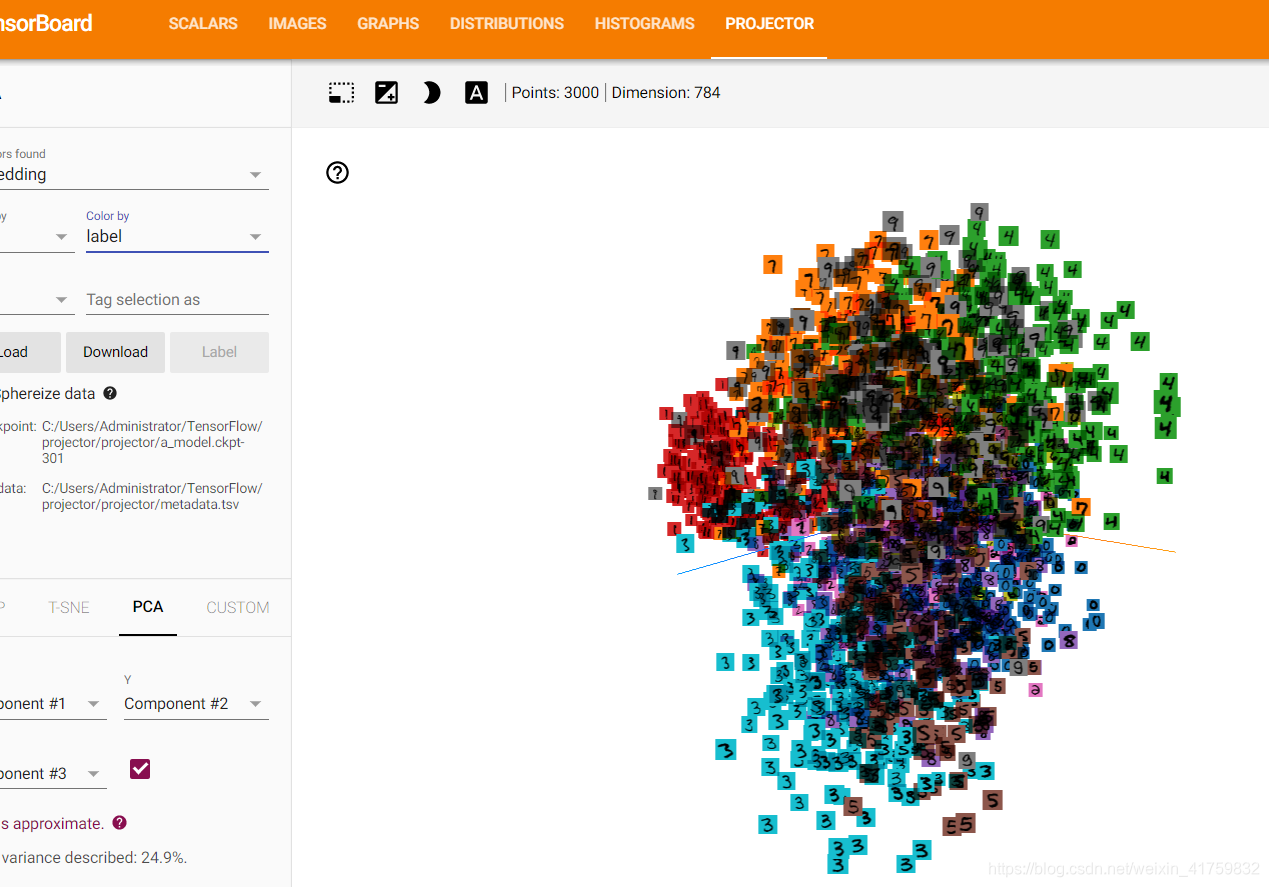
点击T-SNE进行训练然后调整学习率

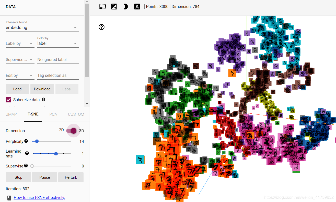
便可得到训练成果。