机器学习学习笔记（四）—— 逻辑回归（分类）问题

分类问题(classification)概述：

The classification problem is just like the regression problem, except that the values we now want to predict take on only a small number of discrete values. For now, we will focus on the binary classification problem in which y can take on only two values, 0 and 1. (Most of what we say here will also generalize to the multiple-class case.)

分类问题和回归问题有一定的相似性，先从简单的问题二元分类问题（binary classification problem） 入手，因为下面会介绍怎么从二元分类问题转化成多元分类问题。

假设函数(hypothesis function)定义: 

Our new form uses the "Sigmoid Function," also called the "Logistic Function":

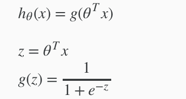
hθ​(x) will give us the probability that our output is 1.

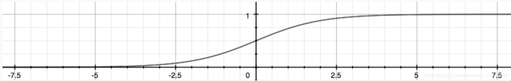
The following image shows us what the sigmoid function looks like:

决策边界（decision boundary）： 

 In order to get our discrete 0 or 1 classification, we can translate the output of the hypothesis function as follows:

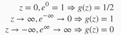
The way our logistic function g behaves is that when its input is greater than or equal to zero, its output is greater than or equal to 0.5:

Remember.

So if our input to g is \theta^T XθTX, then that means:

From these statements we can now say:

The decision boundary is the line that separates the area where y = 0 and where y = 1. It is created by our hypothesis function.

Again, the input to the sigmoid functiondoesn't need to be linear, and could be a function that describes a circle or any shape to fit our data.

逻辑回归模型(logistic regression model)选择/代价函数(cost function)定义 :

逻辑回归模型选择参考这篇博客： https://blog.youkuaiyun.com/saltriver/article/details/63683092

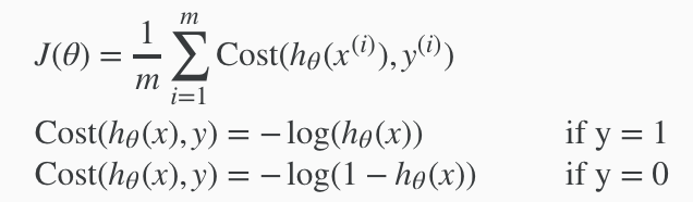
我们选择对数模型。Instead, our cost function for logistic regression looks like: 

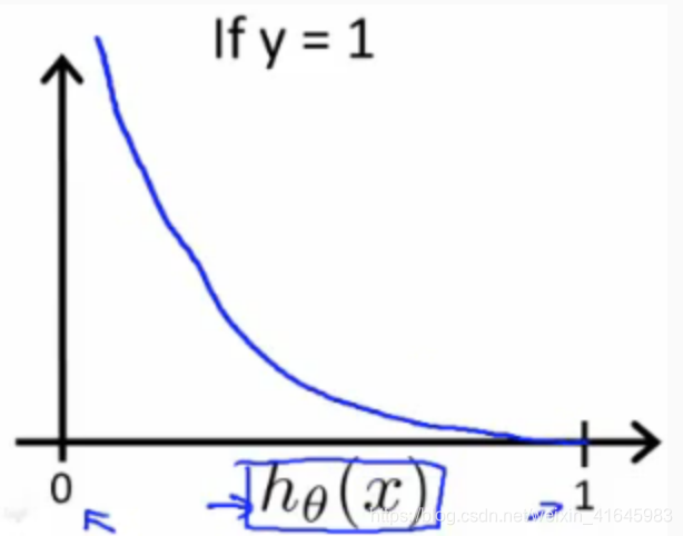
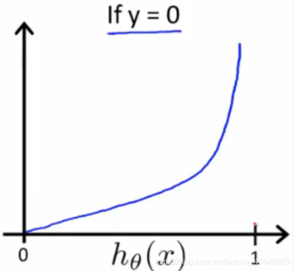
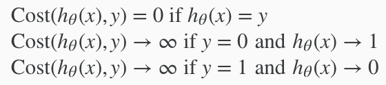
这是一个分段函数，我们可以通过一些技巧合并y=0和y=1这两段函数，从而简化方程式.We can compress our cost function's two conditional cases into one case:

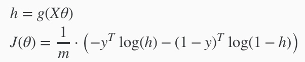
We can fully write out our entire cost function as follows:

A vectorized implementation is:

梯度下降(gradient descent)算法的实现 :

Remember that the general form of gradient descent is:

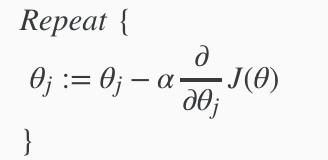
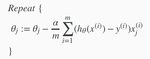
We can work out the derivative part using calculus to get:

注：公式推导参考这篇博客 https://www.jianshu.com/p/610859e27f66

Notice that this algorithm is identical to the one we used in linear regression. We still have to simultaneously update all values in theta.

A vectorized implementation is:

更优化的算法： 

除了梯度下降算法，还有很多更优的算法来解决逻辑回归分类问题。"Conjugate gradient", "BFGS", and "L-BFGS" are more sophisticated, faster ways to optimize θ that can be used instead of gradient descent.  

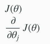
我们只需要提供下面两个输入值，We first need to provide a function that evaluates the following two functions for a given input value θ:

将两个返回值写到一个函数里面，We can write a single function that returns both of these:

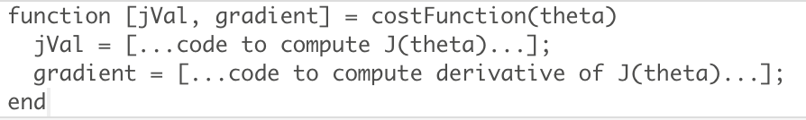
示例代码：

h = sigmoid(X * theta);
J = (-log(h)' * y - log(1 - h)' * (1 - y)) / m;
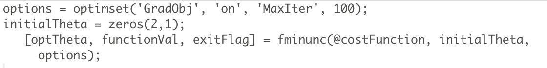
grad = (X' * (h - y)) ./ m;

Octave中实现，Then we can use octave's "fminunc()" optimization algorithm along with the "optimset()" function that creates an object containing the options we want to send to "fminunc()".

示例代码：

%  In this exercise, you will use a built-in function (fminunc) to find the
%  optimal parameters theta.

%  Set options for fminunc
options = optimset('GradObj', 'on', 'MaxIter', 400);

%  Run fminunc to obtain the optimal theta
%  This function will return theta and the cost 
[theta, cost] = ...
	fminunc(@(t)(costFunction(t, X, y)), initial_theta, options);

% Print theta to screen

We give to the function "fminunc()" our cost function, our initial vector of theta values, and the "options" object that we created beforehand.

转化成解决多元分类问题（Multiclass Classification: One-vs-all）： 

Since y = {0,1...n}, we divide our problem into n+1 (+1 because the index starts at 0) binary classification problems; in each one, we predict the probability that 'y' is a member of one of our classes.

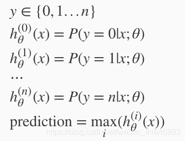
We are basically choosing one class and then lumping all the others into a single second class. We do this repeatedly, applying binary logistic regression to each case, and then use the hypothesis that returned the highest value as our prediction.

当有多个分类时，我们分别选择其中一个分类作为1类，然后将其他的类当成0类，这样计算之后就会有n个h(x)即对于它是(1...n)类的概率，我们选择概率最大的类进行输出。

示例代码:

lambda = 0.1;
for i = 1 : num_labels,
    options = optimset('GradObj', 'on', 'MaxIter', 50);
    initialTheta = zeros(n + 1, 1);
    c = i;
    if c == 10,
        c = 0;
    end;
    theta = fmincg (@(t)(lrCostFunction(t, X, (y == c), lambda)), initialTheta, options);
    all_theta(i, :) = theta';
    % fprintf('%dX%d\n', size(theta, 1), size(theta, 2));
    % fprintf('%dX%d\n', size(all_theta, 1), size(all_theta, 2));
end;