逻辑回归

最新推荐文章于 2022-01-26 18:29:56 发布

CID( ͡ _ ͡°)

最新推荐文章于 2022-01-26 18:29:56 发布

阅读量213

点赞数

CC 4.0 BY-SA版权

分类专栏：机器学习算法

本文链接：https://blog.youkuaiyun.com/weixin_40533189/article/details/90256997

机器学习算法专栏收录该内容

13 篇文章

订阅专栏

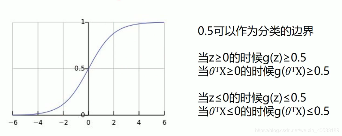
sigmoid / logistic Function

我们定义逻辑回归的预测函数为 $h\Theta (x) = g(\Theta ^{T}x)$ ,其中g(x) 函数是sigmoid函数.

$g(x) = \frac{1}{1+e^{-x}}$ $h\Theta (x) = \frac{1}{1+e^{-\Theta ^{T}X}}$

正确率 / 召回率 / F1指标

正确率与召回率是广泛应用于信息检索和统计学分类领域的两个度量值,用来评估结果的质量

一般来说,正确率就是检索出来的条目有多少正确的,召回率就是所有正确的条目有多少被检索出来了.

F1值 = 2 * (正确率 * 召回率 / 正确率 + 召回率) .是综合上面的两个指标的评估指标,用于综合反映整体的指标.

这几个指标的取值都在 0 - 1之间 , 数值月接近于1 ,效果越好.

梯度下降 - - 逻辑回归

import matplotlib.pyplot as plt
import numpy as np
from sklearn.metrics import classification_report
from sklearn import preprocessing
# 数据是否标准化
scale = False

# 载入数据
data = np.genfromtxt('data.csv',delimiter = ',')
x_data = data[:,:-1]
y_data = data[:,-1]

def plot():
    x0 = []
    x1 = []
    y0 = []
    y1 = []
    #  切分不同类别的数据
    for i in range(len(x_data)):
        if y_data[i] == 0:
            x0.append(x_data[i,0]
            y0.append(x_data[i,1]
        else:
            x1.append(x_data[i,0]
            y1.append(x_data[i,1]
        


        # 画图
        scatter0 = plt.sctter(x0,y0,c='b',marker='o')
        scatter1 = plt.sctter(x1,y1,c='r',marker='x')
        # 画图例
        plt.legend(handles = [scatter0,scatter1],labels = ['label0','label1'],loc='best')
plot()
plt.show()

# 数据处理,添加偏置项
x_data = data[:,:-1]
y_data = data[:,-1,np.newaxis]
print(np.mat(x_data).shape,np.mat(y_data).shape)

# 给样本添加偏置项
X_data = np.concatenate((np.ones((100,1)),x_data),axis = 1)
print(X_data.shape)

def sigmoid(x):
    return 1.0 / (1 + np.exp(-x))

公式: $g(x ) = \frac{1}{1+e^{-x}}$

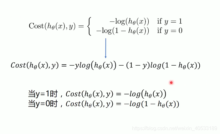
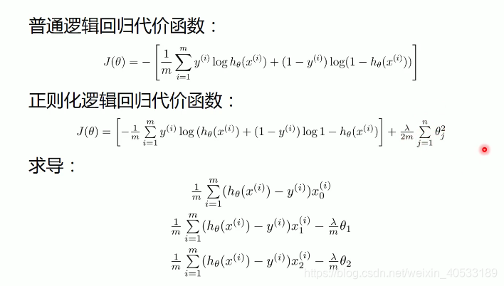
逻辑回归的代价函数
def cost(xMat,yMat,ws):
    left = np.multiply(yMat,np.log(sigmoid(xMat * ws)))
    right = np.multiply(1 - yMat,np.log(sigmoid(xMat * ws)))
    return np.sum(left + right) / -(len(xMat))
$Cost(h\Theta (x),y) = -ylog(h\Theta (x)) - (1-y)log(1-h\Theta (x))$

以上的参数是:

left为上面的公式里面的前半部分也就是: $-ylog(h\Theta (x))$ 的计算

right 为上面的公式里面的后半部分也就是: $- (1-y)log(1-h\Theta (x))$ 的计算

ws 为权值,也就是正则化权重

# 求梯度,然后用梯度来改变权值

def gradAscent(xArr,yArr):
    if scale = True:
        xArr = preprocessing.scale(xArr)
    xMat = np.mat(xArr)
    yMat = np.mat(yArr)
    
    lr = 0.001
    epochs = 10000
    costList = []
    
    # 计算数据行列数
    # 行代表数据个数,列代表权值个数
    m,n = np.shape(xMat)
    # 初始化权值
    ws = np.mat(np.ones((n,1)))
    
    for i in range(epochs + 1):
        # xMat和weights矩阵相乘
        h = sigmoid(xMat * ws)
        # 计算误差
        ws_grad = xMat.T * (h - yMat)/m
        ws = ws - lr * ws_grad
        
        if i % 50 == 0:
            costList.append(cost(xMat,yMat,ws))
    return ws,costList

mat可以从字符串或列表中生成；array只能从列表中生成

sklearn.preprocessing数据标准化的例子:

from sklearn import preprocessing
import numpy as np
x = np.array([[1.,-1.,2.],[2.,0.,0.],[0.,1.,-1.]])
print(preprocessing.scale(x))

[[ 0.         -1.22474487  1.33630621]
 [ 1.22474487  0.         -0.26726124]
 [-1.22474487  1.22474487 -1.06904497]]

标准化的计算方式是: $X_{norm} = \frac{X-X_{mean}}{X_{std}}$

数据集的标准化是许多机器学习估计器的一个常见的要求,如果单个特征看起来不像正太分布数据(例如均值为0的高斯分布和单位方差),他们的性能可能比较差

注意:sklearn里面的sigmoid自带

$wsgrad =\frac{1}{m} \sum_{i=1}^{m} x(h\Theta (x) - y)$

xMat.T 就是把矩阵个转置

# 训练模型,得到权值和cost值的变化
ws,costList = gradAscent(X_data,y_data)
print(ws)

if scale == False:
    # 画图决策边界
    plot()
    x_test = [[-4],[3]]
    y_test = (-ws[0] - x_test * ws[1] ) / ws[2]
    plt.plot(x_test,y_test,'k')
    plt.show()

# 预测
def predict(x_data,ws):
    if scale = True:
        x_data = preprocessing.scale(x_data)
    xMat = np.mat(x_data)
    ws = np.mat(ws)
    return [1 if x>=0.5 else 0 for x in sigmoid(xMat * ws)]
predictions = predict(X_data,ws)
print(classification_report(y_data,predictions))

classification_report :计算准确率,召回率

sklearn实现逻辑回归

import matplotlib.pyplot as plt
import numpy as np
from sklearn.metrics import classification_report
from sklearn import preprocessing
from sklearn import linear_model
# 数据是否需要标准化
scale = False

#载入数据
data = np.genfromtxt('data.csv',delimiter = ',')
x_data = data[:,:-1]
y_data = data[:,-1]

def plot():
    x0 = []
    x1 = []
    y0 = []
    y1 = []
    #切分不同类别的数据
    for i in range(len(x_data)):
        if y_data[i] == 0:
            x0.append(x_data[i,0]
            y0.append(x_data[i,1]
        else:
            x1.append(x_data[i,0]
            y1.append(x_data[i,1]
    # 画图
    scatter0 = plt.scatter(x0,y0,c='b' ,marker='o')
    scatter1 = plt.scatter(x1,y1,c='r',marker = 'x')
    # 画图例
    plt.legend(handles = [scatter0,scatter1],labels = ['label0','label1'],loc = 'best')
plot()
plt.show()

# 定义逻辑回归
logistic = linear_model.LogisticRegression()
logistic.fit(x_data,y_data)

if scale == False:
    plot()
    x_test = np.array([[-4],[3]])
    y_test = (-logistic.intercept_ - x_test * logistic.coef_[0][0]) / logistic.coef_[0][1]
    plt.plot(x_test,y_test,'k')
    plt.show()

# 预测
predictions = logistic.predict(x_data)
print(classification_report(y_data,predicttions)