


 本文详细介绍R语言中lubridate包的使用方法,包括日期时间数据类型的创建、转换、提取和调整,以及如何处理时区和日期时间的数学运算。
R for Data Science总结之——Dates and times
本章介绍lubridate包,可以方便处理日期相关数据分析工作:
library(tidyverse)

library(lubridate)
library(nycflights13)
在R中有三种日期时间相关的数据类型:
- date
- time
- date-time
对于times,可使用hms包
today()
#> [1] "2018-11-19"
now()
#> [1] "2018-11-19 13:40:53 UTC"
也可以通过字符串,或者date-time元素或者date/time类型变量创建。
ymd("2017-01-31")
#> [1] "2017-01-31"
mdy("January 31st, 2017")
#> [1] "2017-01-31"
dmy("31-Jan-2017")
#> [1] "2017-01-31"
也可以不通过字符串直接用数字创建:
ymd(20170131)
#> [1] "2017-01-31"
以上创建的是date类型元素,要创建date-time类型:
ymd_hms("2017-01-31 20:11:59")
#> [1] "2017-01-31 20:11:59 UTC"
mdy_hm("01/31/2017 08:01")
#> [1] "2017-01-31 08:01:00 UTC"
也可以通过tz关键字设置时区:
ymd(20170131, tz = "UTC")
#> [1] "2017-01-31 UTC"
有的时候date-time数据储存在一个数据集的多列之中:
flights %>%
  select(year, month, day, hour, minute)
#> # A tibble: 336,776 x 5
#>    year month   day  hour minute
#>   <int> <int> <int> <dbl>  <dbl>
#> 1  2013     1     1     5     15
#> 2  2013     1     1     5     29
#> 3  2013     1     1     5     40
#> 4  2013     1     1     5     45
#> 5  2013     1     1     6      0
#> 6  2013     1     1     5     58
#> # ... with 3.368e+05 more rows
对于这种情况使用make_date()或make_datetime():
flights %>%
  select(year, month, day, hour, minute) %>%
  mutate(departure = make_datetime(year, month, day, hour, minute))
#> # A tibble: 336,776 x 6
#>    year month   day  hour minute departure
#>   <int> <int> <int> <dbl>  <dbl> <dttm>
#> 1  2013     1     1     5     15 2013-01-01 05:15:00
#> 2  2013     1     1     5     29 2013-01-01 05:29:00
#> 3  2013     1     1     5     40 2013-01-01 05:40:00
#> 4  2013     1     1     5     45 2013-01-01 05:45:00
#> 5  2013     1     1     6      0 2013-01-01 06:00:00
#> 6  2013     1     1     5     58 2013-01-01 05:58:00
#> # ... with 3.368e+05 more rows
通常会编写成函数进行相关操作:
make_datetime_100 <- function(year, month, day, time) {
  make_datetime(year, month, day, time %/% 100, time %% 100)
}

flights_dt <- flights %>%
  filter(!is.na(dep_time), !is.na(arr_time)) %>%
  mutate(
    dep_time = make_datetime_100(year, month, day, dep_time),
    arr_time = make_datetime_100(year, month, day, arr_time),
    sched_dep_time = make_datetime_100(year, month, day, sched_dep_time),
    sched_arr_time = make_datetime_100(year, month, day, sched_arr_time)
  ) %>%
  select(origin, dest, ends_with("delay"), ends_with("time"))

flights_dt
#> # A tibble: 328,063 x 9
#>   origin dest  dep_delay arr_delay dep_time            sched_dep_time
#>   <chr>  <chr>     <dbl>     <dbl> <dttm>              <dttm>
#> 1 EWR    IAH           2        11 2013-01-01 05:17:00 2013-01-01 05:15:00
#> 2 LGA    IAH           4        20 2013-01-01 05:33:00 2013-01-01 05:29:00
#> 3 JFK    MIA           2        33 2013-01-01 05:42:00 2013-01-01 05:40:00
#> 4 JFK    BQN          -1       -18 2013-01-01 05:44:00 2013-01-01 05:45:00
#> 5 LGA    ATL          -6       -25 2013-01-01 05:54:00 2013-01-01 06:00:00
#> 6 EWR    ORD          -4        12 2013-01-01 05:54:00 2013-01-01 05:58:00
#> # ... with 3.281e+05 more rows, and 3 more variables: arr_time <dttm>,
#> #   sched_arr_time <dttm>, air_time <dbl>

flights_dt %>%
  ggplot(aes(dep_time)) +
  geom_freqpoly(binwidth = 86400) # 86400 seconds = 1 day
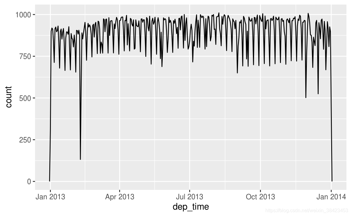
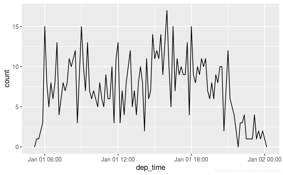
查看单天数据:
flights_dt %>%
  filter(dep_time < ymd(20130102)) %>%
  ggplot(aes(dep_time)) +
  geom_freqpoly(binwidth = 600) # 600 s = 10 minutes
若想将date-time和date类型相互转换,使用as_datetime()或as_date():
as_datetime(today())
#> [1] "2018-11-19 UTC"
as_date(now())
#> [1] "2018-11-19"
所有的日期数据都是按照Unix Epoch也就是1970-01-01开始的,若传入数字则在该时间向上累加:
as_datetime(60 * 60 * 10)
#> [1] "1970-01-01 10:00:00 UTC"
as_date(365 * 10 + 2)
#> [1] "1980-01-01"
可使用year(),month(),mday(),yday(),wday(),hour(),minute(),second()等函数提取相应数据:
atetime <- ymd_hms("2016-07-08 12:34:56")

year(datetime)
#> [1] 2016
month(datetime)
#> [1] 7
mday(datetime)
#> [1] 8

yday(datetime)
#> [1] 190
wday(datetime)
#> [1] 6
对于month()和wday()可以设置label参数显示对应月份和星期几,设置abbr控制是否为全称还是缩写:
month(datetime, label = TRUE)
#> [1] Jul
#> 12 Levels: Jan < Feb < Mar < Apr < May < Jun < Jul < Aug < Sep < ... < Dec
wday(datetime, label = TRUE, abbr = FALSE)
#> [1] Friday
#> 7 Levels: Sunday < Monday < Tuesday < Wednesday < Thursday < ... < Saturday
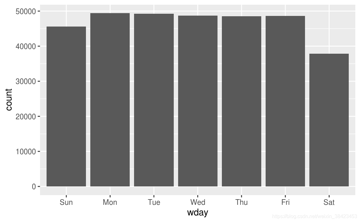
我们可以使用wday()看一周的飞机流量:
flights_dt %>%
  mutate(wday = wday(dep_time, label = TRUE)) %>%
  ggplot(aes(x = wday)) +
    geom_bar()
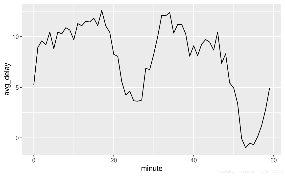
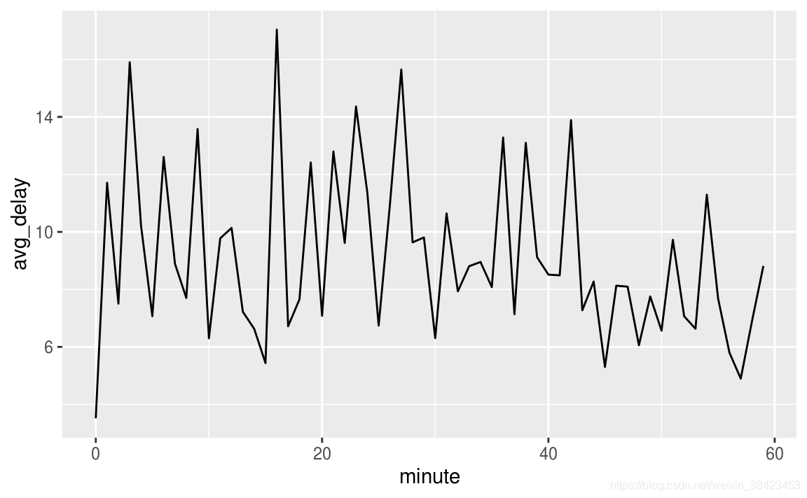
同样可以研究分钟对起飞时间的影响:
flights_dt %>%
  mutate(minute = minute(dep_time)) %>%
  group_by(minute) %>%
  summarise(
    avg_delay = mean(arr_delay, na.rm = TRUE),
    n = n()) %>%
  ggplot(aes(minute, avg_delay)) +
    geom_line()
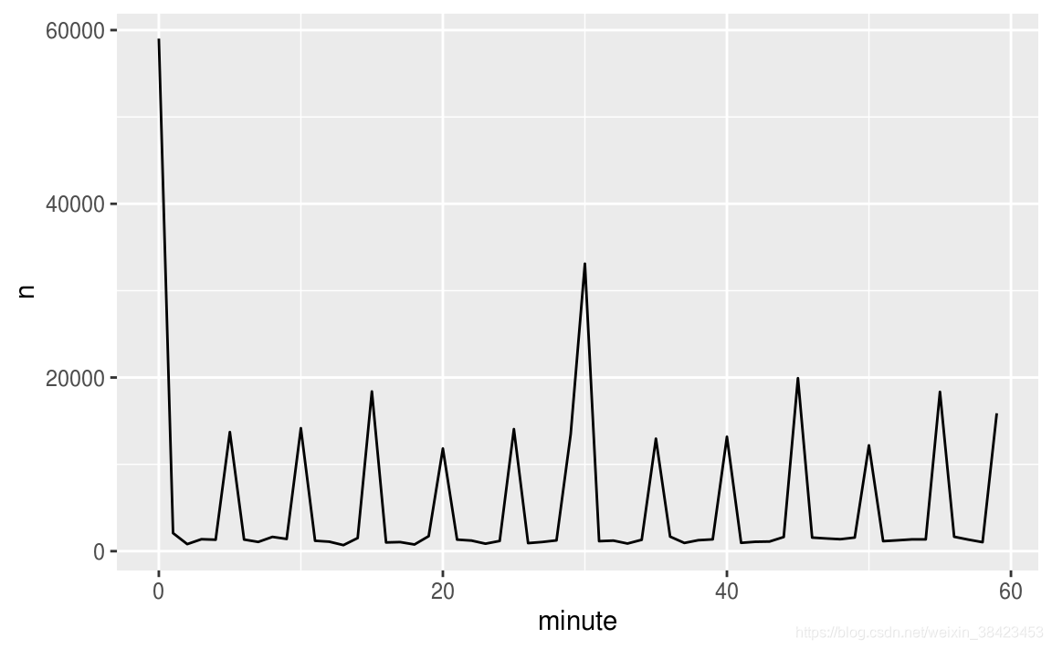
sched_dep <- flights_dt %>%
  mutate(minute = minute(sched_dep_time)) %>%
  group_by(minute) %>%
  summarise(
    avg_delay = mean(arr_delay, na.rm = TRUE),
    n = n())

ggplot(sched_dep, aes(minute, avg_delay)) +
  geom_line()
ggplot(sched_dep, aes(minute, n)) +
  geom_line()
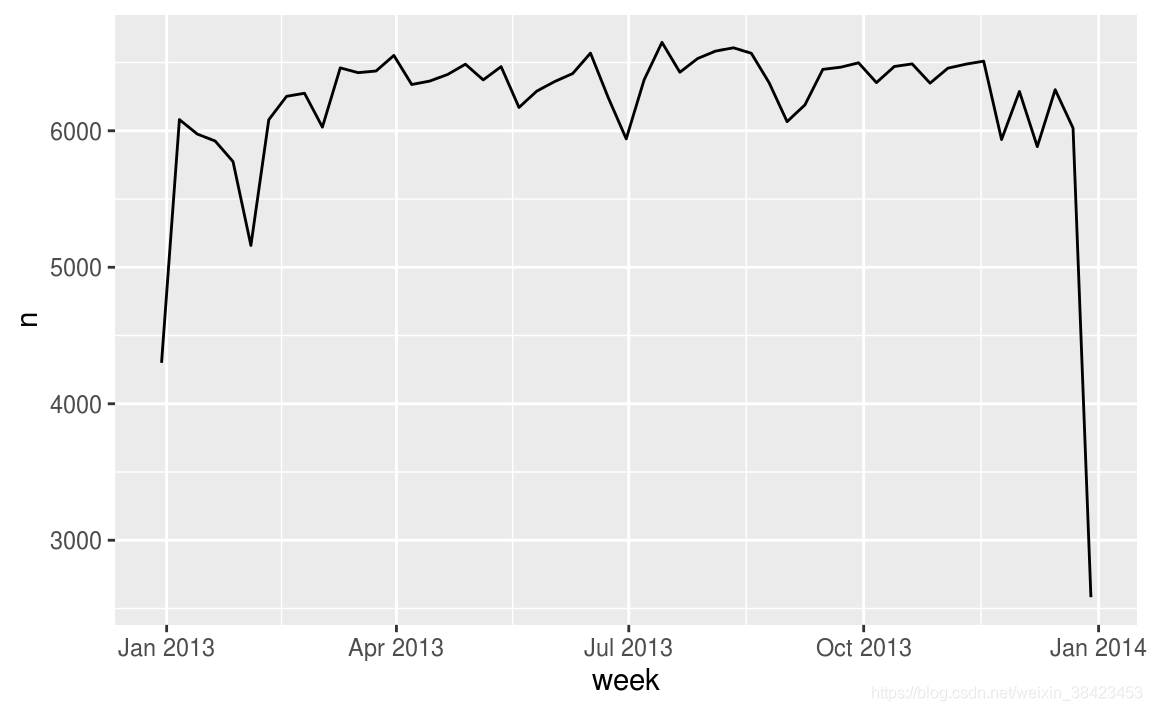
可通过floor_date(),round_date(),ceiling_date()对日期进行四舍五入:
flights_dt %>%
  count(week = floor_date(dep_time, "week")) %>%
  ggplot(aes(week, n)) +
    geom_line()
对日期变量中各个成分进行赋值调整:
(datetime <- ymd_hms("2016-07-08 12:34:56"))
#> [1] "2016-07-08 12:34:56 UTC"

year(datetime) <- 2020
datetime
#> [1] "2020-07-08 12:34:56 UTC"
month(datetime) <- 01
datetime
#> [1] "2020-01-08 12:34:56 UTC"
hour(datetime) <- hour(datetime) + 1
datetime
#> [1] "2020-01-08 13:34:56 UTC"
也可以用update()一次性调整:
update(datetime, year = 2020, month = 2, mday = 2, hour = 2)
#> [1] "2020-02-02 02:34:56 UTC"
当数字太大时会进位:
ymd("2015-02-01") %>%
  update(mday = 30)
#> [1] "2015-03-02"
ymd("2015-02-01") %>%
  update(hour = 400)
#> [1] "2015-02-17 16:00:00 UTC"
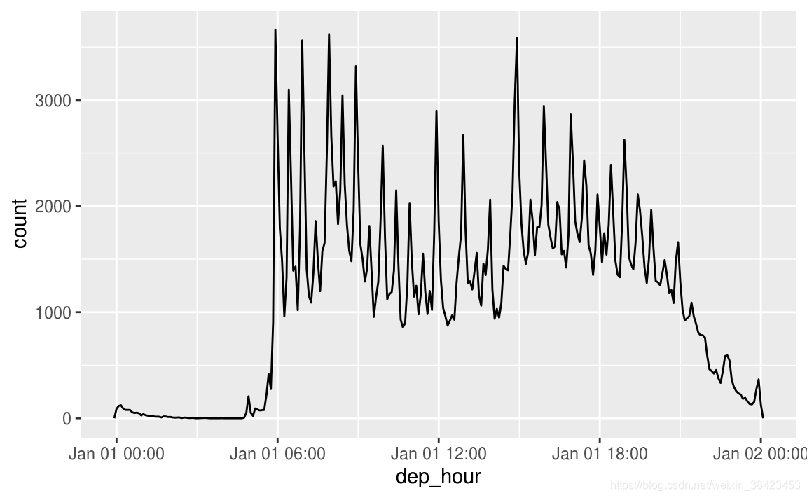
可以通过这个方法将所有飞机起飞时间都改成一天,然后看时辰对起飞时间的影响:
flights_dt %>%
  mutate(dep_hour = update(dep_time, yday = 1)) %>%
  ggplot(aes(dep_hour)) +
    geom_freqpoly(binwidth = 300)
时间范围分为:
- duration:代表用秒表示的确切时间
- period:表示人类单位例如周和月
- interval:开始时间和结束时间
直接两个时间相减结果为:
# How old is Hadley?
h_age <- today() - ymd(19791014)
h_age
#> Time difference of 14281 days
变化为duration:
as.duration(h_age)
#> [1] "1233878400s (~39.1 years)"
这其中有许多子类:
dseconds(15)
#> [1] "15s"
dminutes(10)
#> [1] "600s (~10 minutes)"
dhours(c(12, 24))
#> [1] "43200s (~12 hours)" "86400s (~1 days)"
ddays(0:5)
#> [1] "0s"                "86400s (~1 days)"  "172800s (~2 days)"
#> [4] "259200s (~3 days)" "345600s (~4 days)" "432000s (~5 days)"
dweeks(3)
#> [1] "1814400s (~3 weeks)"
dyears(1)
#> [1] "31536000s (~52.14 weeks)"
可以进行相加减:
2 * dyears(1)
#> [1] "63072000s (~2 years)"
dyears(1) + dweeks(12) + dhours(15)
#> [1] "38847600s (~1.23 years)"

tomorrow <- today() + ddays(1)
last_year <- today() - dyears(1)
由于duration代表确切时间不考虑月份年份时区等的影响,偶尔会得到不可预料的结果:
one_pm <- ymd_hms("2016-03-12 13:00:00", tz = "America/New_York")

one_pm
#> [1] "2016-03-12 13:00:00 EST"
one_pm + ddays(1)
#> [1] "2016-03-13 14:00:00 EDT"
这种时候就需要period:
one_pm
#> [1] "2016-03-12 13:00:00 EST"
one_pm + days(1)
#> [1] "2016-03-13 13:00:00 EDT"
period的表示去掉duration中所有的前缀d:
seconds(15)
#> [1] "15S"
minutes(10)
#> [1] "10M 0S"
hours(c(12, 24))
#> [1] "12H 0M 0S" "24H 0M 0S"
days(7)
#> [1] "7d 0H 0M 0S"
months(1:6)
#> [1] "1m 0d 0H 0M 0S" "2m 0d 0H 0M 0S" "3m 0d 0H 0M 0S" "4m 0d 0H 0M 0S"
#> [5] "5m 0d 0H 0M 0S" "6m 0d 0H 0M 0S"
weeks(3)
#> [1] "21d 0H 0M 0S"
years(1)
#> [1] "1y 0m 0d 0H 0M 0S"
也可以进行加乘运算:
10 * (months(6) + days(1))
#> [1] "60m 10d 0H 0M 0S"
days(50) + hours(25) + minutes(2)
#> [1] "50d 25H 2M 0S"
此时于date类型加减会得到更符合人类认知的结果:
# A leap year
ymd("2016-01-01") + dyears(1)
#> [1] "2016-12-31"
ymd("2016-01-01") + years(1)
#> [1] "2017-01-01"

# Daylight Savings Time
one_pm + ddays(1)
#> [1] "2016-03-13 14:00:00 EDT"
one_pm + days(1)
#> [1] "2016-03-13 13:00:00 EDT"
这可用于对过夜的飞机时间进行修正:
flights_dt %>%
  filter(arr_time < dep_time)
#> # A tibble: 10,633 x 9
#>   origin dest  dep_delay arr_delay dep_time            sched_dep_time
#>   <chr>  <chr>     <dbl>     <dbl> <dttm>              <dttm>
#> 1 EWR    BQN           9        -4 2013-01-01 19:29:00 2013-01-01 19:20:00
#> 2 JFK    DFW          59        NA 2013-01-01 19:39:00 2013-01-01 18:40:00
#> 3 EWR    TPA          -2         9 2013-01-01 20:58:00 2013-01-01 21:00:00
#> 4 EWR    SJU          -6       -12 2013-01-01 21:02:00 2013-01-01 21:08:00
#> 5 EWR    SFO          11       -14 2013-01-01 21:08:00 2013-01-01 20:57:00
#> 6 LGA    FLL         -10        -2 2013-01-01 21:20:00 2013-01-01 21:30:00
#> # ... with 1.063e+04 more rows, and 3 more variables: arr_time <dttm>,
#> #   sched_arr_time <dttm>, air_time <dbl>
对过夜飞机的到达时间进行日期加1:
flights_dt <- flights_dt %>%
  mutate(
    overnight = arr_time < dep_time,
    arr_time = arr_time + days(overnight * 1),
    sched_arr_time = sched_arr_time + days(overnight * 1)
  )
这就修正了数据集:
flights_dt %>%
  filter(overnight, arr_time < dep_time)
#> # A tibble: 0 x 10
#> # ... with 10 variables: origin <chr>, dest <chr>, dep_delay <dbl>,
#> #   arr_delay <dbl>, dep_time <dttm>, sched_dep_time <dttm>,
#> #   arr_time <dttm>, sched_arr_time <dttm>, air_time <dbl>,
#> #   overnight <lgl>
duration和period的主要区别在于,period会随年份变化变化时间区间:
years(1) / days(1)
#> estimate only: convert to intervals for accuracy
#> [1] 365
如果想获得精确衡量则需要interval:
next_year <- today() + years(1)
(today() %--% next_year) / ddays(1)
#> [1] 365

(today() %--% next_year) %/% days(1)
#> Note: method with signature 'Timespan#Timespan' chosen for function '%/%',
#>  target signature 'Interval#Period'.
#>  "Interval#ANY", "ANY#Period" would also be valid
#> [1] 365
时区:
Sys.timezone()
#> [1] "UTC"
查看所有时区:
length(OlsonNames())
#> [1] 606
head(OlsonNames())
#> [1] "Africa/Abidjan"     "Africa/Accra"       "Africa/Addis_Ababa"
#> [4] "Africa/Algiers"     "Africa/Asmara"      "Africa/Asmera"
在R中,时区时date-time类型变量的一个属性:
(x1 <- ymd_hms("2015-06-01 12:00:00", tz = "America/New_York"))
#> [1] "2015-06-01 12:00:00 EDT"
(x2 <- ymd_hms("2015-06-01 18:00:00", tz = "Europe/Copenhagen"))
#> [1] "2015-06-01 18:00:00 CEST"
(x3 <- ymd_hms("2015-06-02 04:00:00", tz = "Pacific/Auckland"))
#> [1] "2015-06-02 04:00:00 NZST"
x1 - x2
#> Time difference of 0 secs
x1 - x3
#> Time difference of 0 secs
不出意外的话R永远使用UTC时区:
x4 <- c(x1, x2, x3)
x4
#> [1] "2015-06-01 12:00:00 EDT" "2015-06-01 12:00:00 EDT"
#> [3] "2015-06-01 12:00:00 EDT"
若想保持时间不变更改时区:
x4a <- with_tz(x4, tzone = "Australia/Lord_Howe")
x4a
#> [1] "2015-06-02 02:30:00 +1030" "2015-06-02 02:30:00 +1030"
#> [3] "2015-06-02 02:30:00 +1030"
x4a - x4
#> Time differences in secs
#> [1] 0 0 0
保持数值不变改变时区:
x4b <- force_tz(x4, tzone = "Australia/Lord_Howe")
x4b
#> [1] "2015-06-01 12:00:00 +1030" "2015-06-01 12:00:00 +1030"
#> [3] "2015-06-01 12:00:00 +1030"
x4b - x4
#> Time differences in hours
#> [1] -14.5 -14.5 -14.5
所有代码已上传GITHUB点此进入


 1698
1698

 被折叠的 条评论
为什么被折叠?
被折叠的 条评论
为什么被折叠?
 到【灌水乐园】发言


