


Exercise: Jupyter
Part 1
For each of the four datasets...
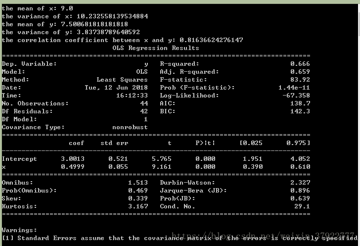
- Compute the mean and variance of both x and y
- Compute the correlation coefficient between x and y
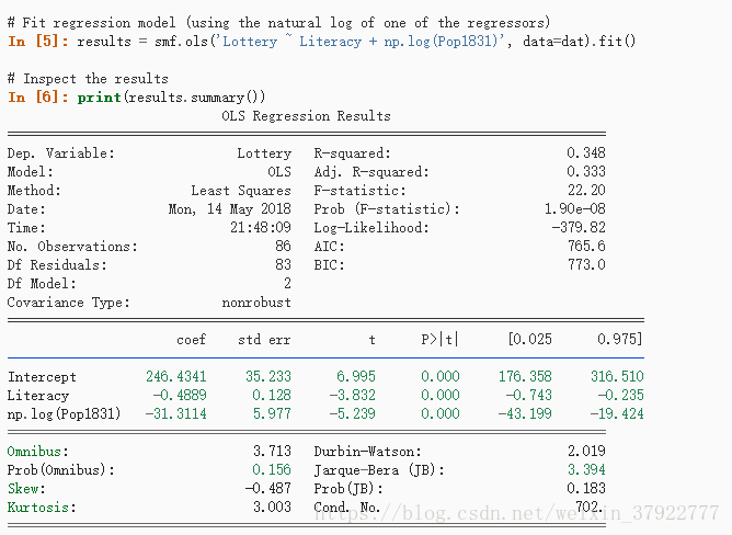
- Compute the linear regression line: y=β0+β1x+ϵy=β0+β1x+ϵ (hint: use statsmodels and look at the Statsmodels notebook)
函数参考网址:
https://www.statsmodels.org/stable/index.html
https://pandas.pydata.org/pandas-docs/stable/api.html
pandas.DataFrame.add
-
Addition of dataframe and other, element-wise (binary operator add).
Equivalent to
dataframe + other, but with support to substitute a fill_value for missing data in one of the inputs.Parameters: -
other
:
Series, DataFrame, or constant
axis : {0, 1, ‘index’, ‘columns’}
For Series input, axis to match Series index on
level : int or name
Broadcast across a level, matching Index values on the passed MultiIndex level
fill_value : None or float value, default None
Fill existing missing (NaN) values, and any new element needed for successful DataFrame alignment, with this value before computation. If data in both corresponding DataFrame locations is missing the result will be missing
Returns: -
result
:
DataFrame
DataFrame.
add
(
other,
axis='columns',
level=None,
fill_value=None
)
[source]
程序实现:
import random
import numpy as np
import scipy as sp
import pandas as pd
import matplotlib.pyplot as plt
import seaborn as sns
import statsmodels.api as sm
import statsmodels.formula.api as smf

# Part 1
# For each of the four datasets...
sns.set_context("talk")
anascombe = pd.read_csv('anscombe.csv')

# Compute the mean and variance of both x and y
x = anascombe.x
y = anascombe.y

mean_x = x.mean()
mean_y = y.mean()
variance_x = x.var()
variance_y = y.var()

print('the mean of x:', str(mean_x))
print('the variance of x:', str(variance_x))
print('the mean of y:', str(mean_y))
print('the variance of y:', str(variance_y))

# Compute the correlation coefficient between x and y
coefficient = x.corr(y, method='pearson', ) #pearson : standard correlation coefficient
print('the correlation coefficient between x and y:', str(coefficient))

# Compute the linear regression line: $y = \beta_0 + \beta_1 x + \epsilon$
res = smf.ols('y~x', data=x.add(y)).fit()
print(res.summary())
结果输出:
Part 2
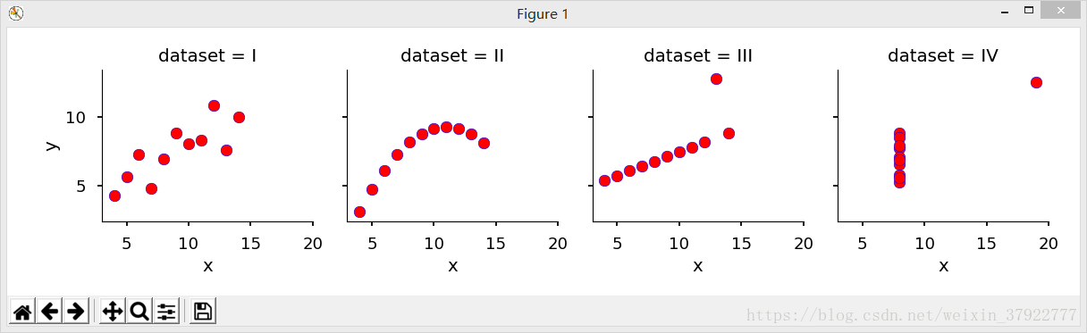
Using Seaborn, visualize all four datasets.
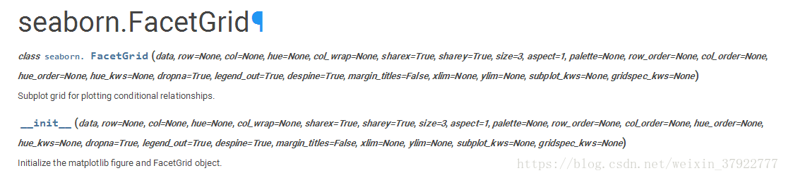
hint: use sns.FacetGrid combined with plt.scatter
函数参考网址:
https://seaborn.pydata.org/generated/seaborn.FacetGrid.html
import scipy as sp
import pandas as pd
import matplotlib.pyplot as plt
import seaborn as sns
import statsmodels.api as sm
import statsmodels.formula.api as smf

# Part 2
sns.set_context("talk")
anascombe = pd.read_csv('anscombe.csv')
# Using Seaborn, visualize all four datasets
g = sns.FacetGrid(anascombe, col="dataset")
g = g.map(plt.scatter, "x", "y", color="r", edgecolor="b")
plt.show()
结果输出:


 被折叠的 条评论
为什么被折叠?
被折叠的 条评论
为什么被折叠?
 到【灌水乐园】发言


