


 本文深入解析K-means聚类算法,涵盖其定义、目的、原理、步骤及弊端解决方案,同时探讨了聚类算法的分类,包括分区、层次、基于图、基于模型及其他类型。文中还介绍了欧几里得距离、Manhattan距离、PCA降维等关键概念,并提供了Python代码实例。
k-means 案例实操
先来看下Clustering Algorithms聚类算法的分类:
1.Partitioning:
Construct k partitions and iteratively update the partitions
(1)k-means(k-均值)
(2) k-medoids(k-中心点)
2.Hierarchical:(层次聚类)
Create a hierarchy of clusters (dendrogram 树状图)
(1)Agglomerative clustering (bottom-up)
(2)Conglomerative clustering (top-down)
3.Graph-based clustering:
Graph-cut algorithms (Spectral Clustering)
4.Model-based clustering
Mixture of Gaussians
5.Other types:
(1)Non-parametric Bayesian (Latent Dirichlet Allocation)
(2)Expectation Maximisation (EM) algorithm
(3)and many more …
k-means(k-均值)
定义
聚类是一个将数据集中在某些方面相似的数据成员进行分类组织的过程,聚类就是一种发现这种内在结构的技术,是无监督学习
目的
给无标签的数据 (或者称为 instance) 分类
宏观来说这个算法是用来干什么的:
- 通过 训练数据集(train dataset) 和 k-means算法 找到每个分类的中心点(cluster centre)
- 在测试或应用时,计算 测试数据点 或 应用数据点(instance) 距离各个分类中心点的距离
- 测试数据或应用数据 距离哪个点最近,就被分到哪一类去
所以,这个算法要做的就是怎么通过训练数据集找到这些分类的中心点
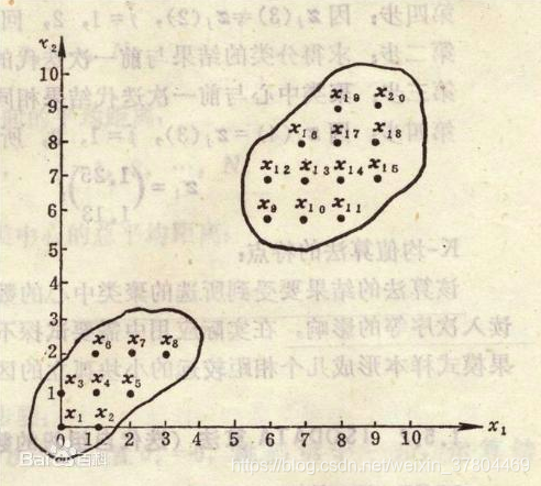
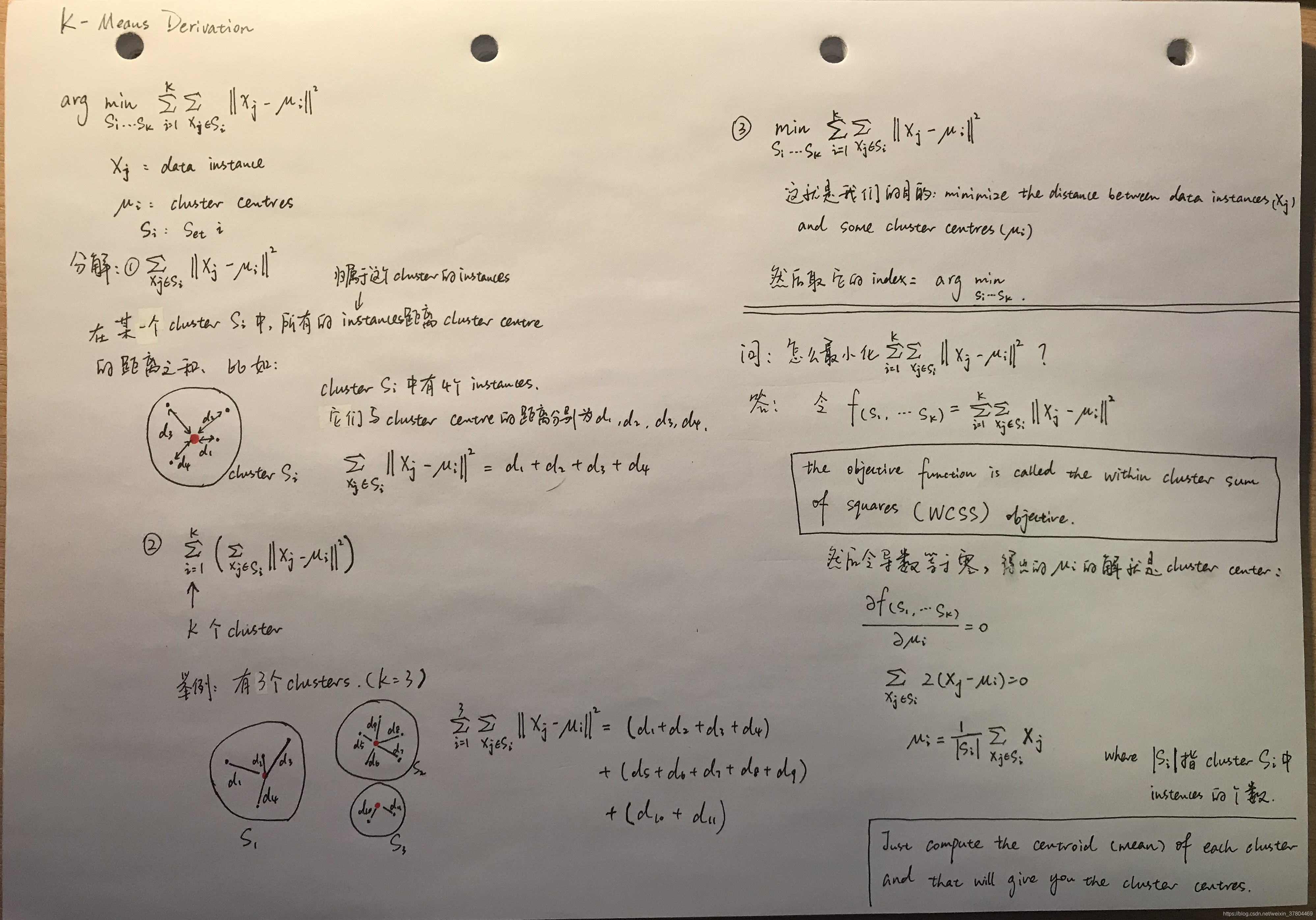
原理 --找聚类中心(cluster centre)
我们要做的就是最小化下面的那个公式
公式的意义: 假如所有的点都被分到了正确的类中,那么所有的点到他们所归属的类中心的距离之和是最小的
步骤
- Input
- cluster 的个数k
- 含有N 个instances的数据集 S = {x1, …, xN}, 每个instance都是 d 维 的实数向量(xi ∈ Rd),代表instance的d个特征(features)
- 从数据集中随机取 k个instances(用于初始化cluster centres,显然每个instance 代表一个cluster centre)
- 将其余的instances分类于与其最近的cluster(计算每个instance与k个cluster centres 的距离,将其归类于距离最小的那个cluster)
- 计算每个cluster里所有instances的平均值,更新cluster centre
- 在第2步,第3步重复,直到收敛(收敛:在做第2步,第2步时,所有点的分类都不再改变)
k-means 算法的弊端及解决方案
-
结果非常依赖初始化时随机选择,或者说 受初始化时选择k个点的影响特别大
-
可能某个分类被圈在一个很小的局部范围,并不是全局最优
解决方案:用不同的初始化数据(k个数据),重复聚类过程多次,并选择最佳的最终聚类。那怎么评估聚类的好坏呢?例如,评估维度有:(下一个模块有详细讲解)
– 1. smallest number of iterations before convergence
在聚类中心值收敛前,使用了最少迭代次数
– largest total distance between the final cluster means
最终的的cluster means值相加,值最大,也就是说聚类中心点之间的距离越大越好 -
离群值对平均值的影响非常大
-
聚类中心(means)不是集群中的点
解决方案:从每个分类中,分别选择其中数据作为初始化聚类中心
涉及知识点
1. 欧几里得距离(Euclidean Distance)
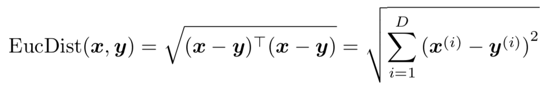
import numpy as np

p1 = np.array([1,2,3])
p2 = np.array([4,5,6])

sum = 0
for i in range(len(p1)):
    sum += pow(p2[i]-p1[i],2)
dis = np.sqrt(sum)

print(dis)

#5.196152422706632
2. Manhatten距离
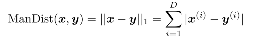
    def distManhatten(self, x, y):
        distance = sum(abs(x-y))
        return distance
3. 降维:PCA(Principal Component Analysis)
如果数据features太多(维度很多),需要进行降维处理,降到二维或三维,方便进行图像输出,具体理论介绍在这里
例子实现二维降到一维
import numpy as np


data = np.array([[0.9, 1.0],
                 [2.4, 2.6],
                 [1.2, 1.7],
                 [0.5, 0.7],
                 [0.3, 0.7],
                 [1.8, 1.4],
                 [0.5, 0.6],
                 [0.3, 0.6],
                 [2.5, 2.6],
                 [1.3, 1.1]])

# 各元素与平均值的差值 (defferences)
X = data - np.reshape(np.mean(data,axis=0),(-1,data.shape[1]))

# 协方差矩阵(coveriance  matrix )
C = (1/data.shape[0]) * np.dot(X.transpose(),X)

# 特征值(eigenValues)与 特征向量(eigenVectors)
eigenValues, eigenVectors = np.linalg.eigh(C)
print('\neigenValues =', np.round(eigenValues, 2))
print('\neigenVectors =', eigenVectors)

# 取最大特征值对应的特征向量 叫"转换矩阵"
U = (eigenVectors[:, np.argsort(-eigenValues)[0:1]])
print('\nU =', U)

# Principal Component 主成分
PCA = np.dot(X,U).transpose()
print('\nPCA :', PCA)


# eigenValues = [0.03 1.13]
#
# eigenVectors = [[ 0.68075138 -0.73251454]
#                 [-0.73251454 -0.68075138]]
#
# U = [[-0.73251454]
#      [-0.68075138]]
#
# PCA : [[ 0.40200434 -1.78596968 -0.29427599  0.89923557  1.04573848 -0.5295593 # 0.96731071  1.11381362 -1.85922114  0.04092339]]
k-means 聚类算法衡量指标
(聚类效果的评价方式大体上可分为性能度量和距离计算两类。)
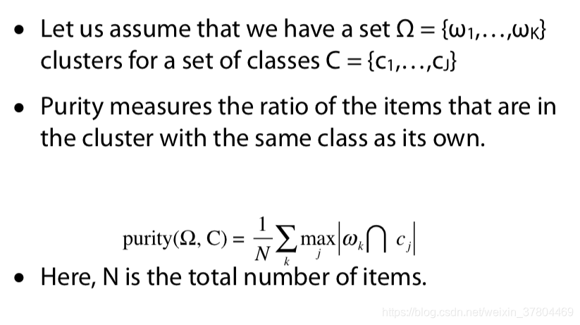
1.purity(纯度)
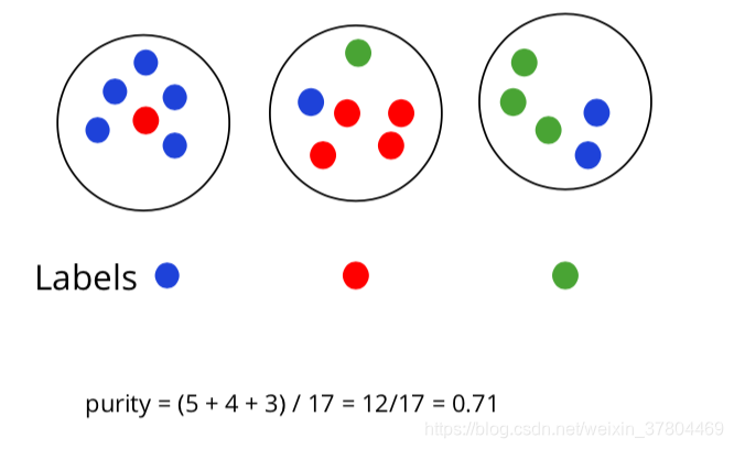
cluster中点最多的那个颜色,定为这个cluster的label。在这个cluster 中和label色不同的点,是错误分类。
栗子:
2.NMI : Normalised Mutual Information (归一化互信息)
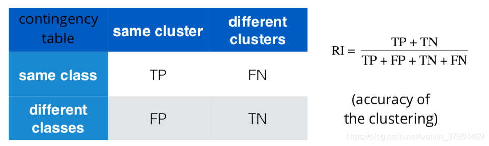
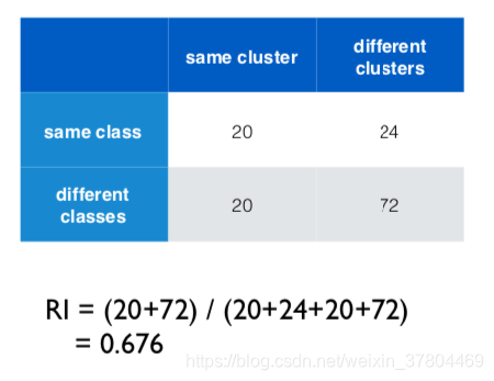
3.Rand index (RI)
- Positive = same cluster
- Negative = different clusters
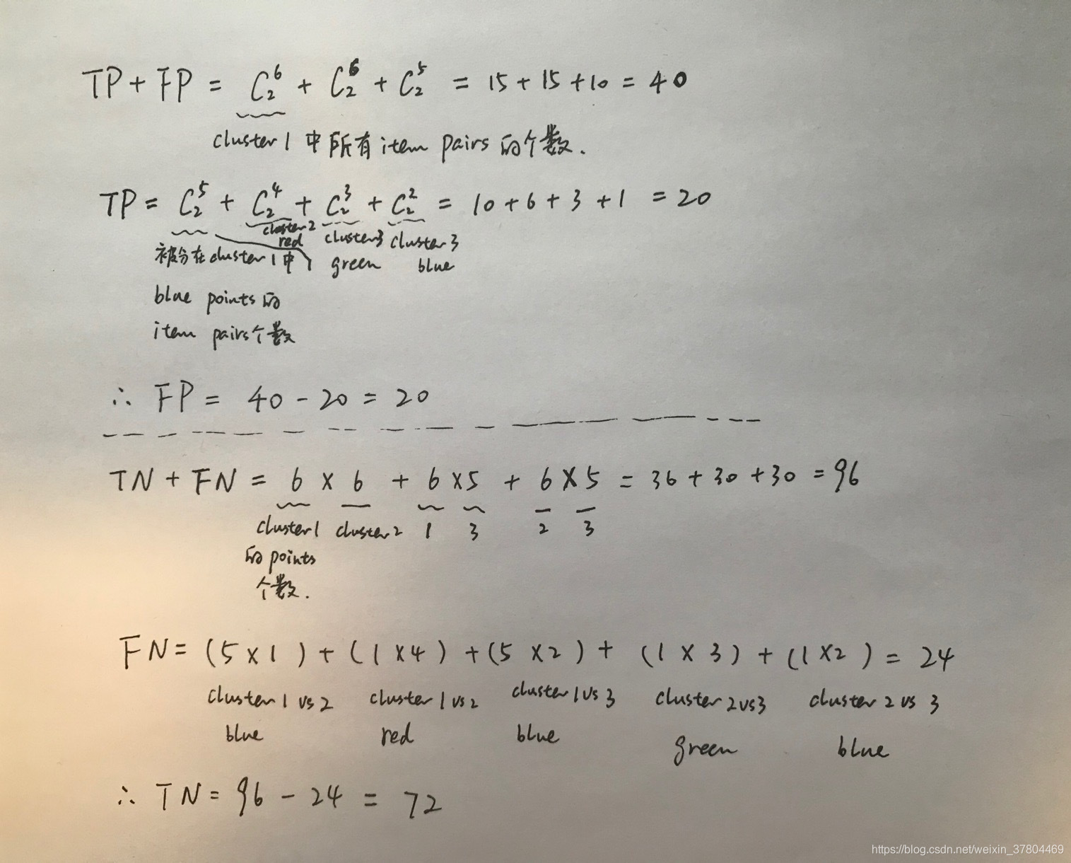
- TP = No. of item pairs that are in the same cluster and belong to the same class
- FP = No. of item pairs that are in the same cluster but belong to different classes
- TN = No. of item pairs that are in different clusters and belong to different classes
- FN = No. of item pairs that are in different clusters but belong to the same class
总结下来可以理解为,positive是分在了同一个cluster, negative是分在了不同的cluster。Ture 和 False 指紧跟它的P 和 N 是分类正确还是错误。
相同的例子:
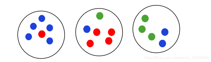
TP + FP: 是不管分类是否正确,被分在了同一个cluster的item pairs
TP: 同一个class的点被正确的分在了同一个cluster中
TN + FN:是不管分类是否正确,被分在了不同的cluster的item pairs
FN:同一个class的点被正确的分在了不同的cluster中
3. P (precision) / R (recall) / F (F-measure)
- P = TP / (TP + FP)
- R = TP / (TP + FN)
- F = 2PR / (P + R)
用上面的例子,以及我们在 RI 中得出的的 TP、FP、TN、FN 的值,计算得出:
- P = TP / (TP+FP) =20 / (20+20) = 0.5
- R = TP / (TP + FN) = 20 / (20 + 24) = 0.45
- F = 2PR / (P + R) = 0.47


 1万+
1万+

 被折叠的 条评论
为什么被折叠?
被折叠的 条评论
为什么被折叠?
 到【灌水乐园】发言


