


原文:Basic classification: Classify images of clothing (https://tensorflow.google.cn/tutorials/keras/classification)
本文是官方教程的翻译,如有错误希望留言指出,能力有限,希望交流。
疫情当前,希望早日战胜疫情。中国加油,武汉加油。
这个教程会教大家训练一个服装图片分类的模型,比如球鞋和球衣。你现在不了细节也不用担心,先让我们快速的过一下 TensorFlow 编程的过程,细节会边过边说,边贴代码。
这个教程使用的是TensorFlow高级API Keras(keras是啥?嗯好问题)。
导入依赖库
from __future__ import absolute_import, division, print_function, unicode_literals# 导入 TensorFlow 和 tf.kerasimport tensorflow as tffrom tensorflow import keras# 依赖库import numpy as npimport matplotlib.pyplot as plt#这里使用的tf2.0新的版本print(tf.__version__)导入Fashion MNIS数据集
这个教程使用的Fashion MNIST数据集包含 7万张灰度图片,又是个分类。每个图片的尺寸是28X28。数据集地址:https://github.com/zalandoresearch/fashion-mnist
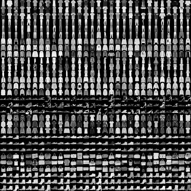
Fashion MNIST数据集
Fashion MNIST目标是取代MNIST数据集。MNIST数据集一般作为机器视觉领域的入门数据集,就像”Hello, World“。MNIST数据集包含的是10数字的手写数据集图片,尺寸和格式和这里使用的样本一样。
Fashion MNIST数据集非常丰富,也比使用传统的MNIST更有意思。这两个数据集都比较小,所以非常适合用来验证算法是不是达到预期。比如适合入门,无压力。
这个例子里,6万图片作为训练集,1万图片作为验证集来验证分类模型的准确度。你可以直接从TensorFlow加载和访问Fashion MNIST 数据集。
fashion_mnist = keras.datasets.fashion_mnist(train_images, train_labels), (test_images, test_labels) = fashion_mnist.load_data()Downloading data from https://storage.googleapis.com/tensorflow/tf-keras-datasets/train-labels-idx1-ubyte.gz32768/29515 [=================================] - 0s 11us/stepDownloading data from https://storage.googleapis.com/tensorflow/tf-keras-datasets/train-images-idx3-ubyte.gz26427392/26421880 [==============================] - 6s 0us/stepDownloading data from https://storage.googleapis.com/tensorflow/tf-keras-datasets/t10k-labels-idx1-ubyte.gz8192/5148 [===============================================] - 0s 0us/stepDownloading data from https://storage.googleapis.com/tensorflow/tf-keras-datasets/t10k-images-idx3-ubyte.gz4423680/4422102 [==============================] - 2s 0us/step加载数据返回NumPy数组。
train_images 和 train_labels 数组是用来训练模型的训练集。test_images 和 test_labels 数组是用来沿验证模型的验证集。这些图片都是 28X28大小的 NumPy arrays形式,每个像素使用0到255的数值代表。”标签“是由从0到9的整数组成的数组。这些数字表示样本服装的分类,如下:
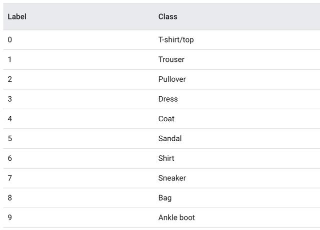
图片对应一个标签。但是数据集中并没有标注类名,所以将类名声明在这里:
class_names = ['T-shirt/top', 'Trouser', 'Pullover', 'Dress', 'Coat', 'Sandal', 'Shirt', 'Sneaker', 'Bag', 'Ankle boot']浏览数据
在训练模型之前先看看数据的格式。下面显示了在数据集中有6万个图片样本。每个图片包含28X28个像素。
train_images.shape(60000, 28, 28)同样的,在训练集中也有6万个标签。
len(train_labels60000每个标签都都是0到9中的一个整数。
train_labelsarray([9, 0, 0, ..., 3, 0, 5], dtype=uint8)验证集中有1万个图片样本,每个也是28X28像素。
test_images.shape(10000, 28, 28)测试集汇中有1万个标签。
len(test_labels)10000数据预处理
在训练模型前,需要把数据预处理一下。如果你检查一下训练集中的第一样本,可以看到像素值都在0到255之间。
plt.figure()plt.imshow(train_images[0])plt.colorbar()plt.grid(False)plt.show()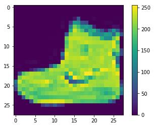
在把数据喂给神经网络模型之前,先把数值缩放到0到1之间。所以,把数值除以255.一定要记住,训练集和测试集一定做同样的操作。
train_images = train_images / 255.0test_images = test_images / 255.0验证一下数据是否格式正确,这样就可以开始构建模型。显示前25个训练集中的样本,在下面显示每个分类的名字。
plt.figure(figsize=(10,10))for i in range(25): plt.subplot(5,5,i+1) plt.xticks([]) plt.yticks([]) plt.grid(False) plt.imshow(train_images[i], cmap=plt.cm.binary) plt.xlabel(class_names[train_labels[i]])plt.show()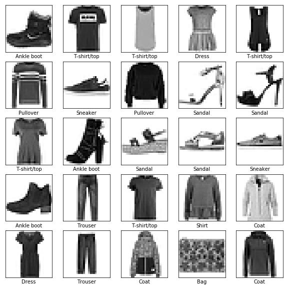
构建模型
要构建模型首先要配置模型各层,然后将模型进行编译。
安装层
神经网络基础的组成部分就是”层“。这些层从喂入的数据中提取特征,并希望这些提特征对于要解决的问题是有用的。
大部分的深度学习都是把简单的层连在一起。大多数层,比如'tf.keras.layers.Dense',都有在训练中学习的参数。
model = keras.Sequential([ keras.layers.Flatten(input_shape=(28, 28)), keras.layers.Dense(128, activation='relu'), keras.layers.Dense(10)])神经网络的第一层`tf.keras.layers.Flatten`,将会把图片的样本格式要从两维数组(28X28 像素)转换成一维数组( 28 X 28 = 784)。可以想象成为这层把图片里的项目一行一行的拼接在一起。这一层没有学习参数,只是改变数据格式。
将像素压平后,这个网络里将是包含由两个全连接层`tf.keras.layers.Dense`组成的序列。这两个层实现全连接。第一个全连接层包含128个神经元节点,第二个层是包含10个节点的softmax层,这个层将返回长度为10的数组,每个数值代表当前图片属于十个分类中每一类的可能性评分,和为1。
编译模型
在训练模型之前,还需要稍微设置一下。这些设置在模型编译这一步进行:
- 损失函数 - 用来衡量训练过程中模型的准确度。通过最小化这个函数的值,来使模型向正确的方向拟合。
- 优化器 — 基于喂入的数据和损失函数来更新模型的参数。
- 评估指标 —用来监控模型训练和验证步骤。例子中使用”准确度“作为来衡量图片被正确分类的分数。
model.compile(optimizer='adam', loss=tf.keras.losses.SparseCategoricalCrossentropy(from_logits=True), metrics=['accuracy'])训练模型
训练模型需要以下步骤:
- 将训练集喂给模型。例子中训练数据就是 `train_images` 和 `train_labels`数组中的数据。
- 模型学习拟合图片和分类标签。
- 让模型去预测`test_images` 数组中的测试集样本。
- 通过比较预测结果和`test_labels`数组中的标签进行评估。
开始训练
通过调用 `model.fit`函数开始训练。
model.fit(train_images, train_labels, epochs=10)Train on 60000 samplesEpoch 1/1060000/60000 [==============================] - 6s 98us/sample - loss: 0.4989 - accuracy: 0.8248Epoch 2/1060000/60000 [==============================] - 5s 78us/sample - loss: 0.3778 - accuracy: 0.8640Epoch 3/1060000/60000 [==============================] - 5s 82us/sample - loss: 0.3381 - accuracy: 0.8763Epoch 4/1060000/60000 [==============================] - 5s 83us/sample - loss: 0.3115 - accuracy: 0.8857Epoch 5/1060000/60000 [==============================] - 5s 84us/sample - loss: 0.2933 - accuracy: 0.8915Epoch 6/1060000/60000 [==============================] - 5s 81us/sample - loss: 0.2795 - accuracy: 0.8967Epoch 7/1060000/60000 [==============================] - 5s 81us/sample - loss: 0.2683 - accuracy: 0.9008Epoch 8/1060000/60000 [==============================] - 5s 81us/sample - loss: 0.2540 - accuracy: 0.9060Epoch 9/1060000/60000 [==============================] - 5s 77us/sample - loss: 0.2454 - accuracy: 0.9070Epoch 10/1060000/60000 [==============================] - 5s 78us/sample - loss: 0.2377 - accuracy: 0.9117在模型训练过程中,损失和准去度评估数值会显示出来。这个模型在训练集上可以达到91%的准确度。
评估准确度
接下来,比较一下在测试集上的表现:
test_loss, test_acc = model.evaluate(test_images, test_labels, verbose=2)print('Test accuracy:', test_acc)10000/10000 - 1s - loss: 0.3340 - accuracy: 0.8840Test accuracy: 0.884可以看出来,在测试集上的表现不如在训练集。测试集和训练集的准确度的差距代表出现了”过拟合“。过拟合是指模型遇到新数据是的性能表现差(兼容性、鲁棒性差)。更多信息:
模型预测输出
模型训练好了,可用用它来预测一些图片:
模型的的线性输出,通过一个softmax层转换成更容易理解的概率可能性。
probability_model = tf.keras.Sequential([model, tf.keras.layers.Softmax()])predictions = probability_model.predict(test_images)看看模型预测的测试集标签:
predictions[0]array([1.4332510e-06, 1.6598245e-08, 1.9020067e-07, 9.7645436e-10, 3.3300270e-07, 9.3532652e-03, 2.0751942e-08, 1.7628921e-02, 1.3357820e-07, 9.7301573e-01], dtype=float32)一个预测结果是一个包括10个数字的数组。这些数字代表了模型认为这些图片数据不通分类的"可信度"。你这样可以找出哪个标签最高:
np.argmax(predictions[0])9
所以,模型认为这个图片最有可能的是“ankle”或者说是 class_names[9]。再看下正确的标签,模型预测对了!
test_labels[0]9将十个分类的预测值绘制出来:
def plot_image(i, predictions_array, true_label, img): predictions_array, true_label, img = predictions_array, true_label[i], img[i] plt.grid(False) plt.xticks([]) plt.yticks([]) plt.imshow(img, cmap=plt.cm.binary) predicted_label = np.argmax(predictions_array) if predicted_label == true_label: color = 'blue' else: color = 'red' plt.xlabel("{} {:2.0f}% ({})".format(class_names[predicted_label], 100*np.max(predictions_array), class_names[true_label]), color=color)def plot_value_array(i, predictions_array, true_label): predictions_array, true_label = predictions_array, true_label[i] plt.grid(False) plt.xticks(range(10)) plt.yticks([]) thisplot = plt.bar(range(10), predictions_array, color="#777777") plt.ylim([0, 1]) predicted_label = np.argmax(predictions_array) thisplot[predicted_label].set_color('red') thisplot[true_label].set_color('blue')验证预测
用训练的模型 在做一些预测看看:
看看第一个图片、预测结果和预测数组。正确的预测标签使用蓝色,错误的有内测使用红色。标签预测的通过百分比数值的形式给出。
i = 0plt.figure(figsize=(6,3))plt.subplot(1,2,1)plot_image(i, predictions[i], test_labels, test_images)plt.subplot(1,2,2)plot_value_array(i, predictions[i], test_labels)plt.show()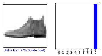
i = 12plt.figure(figsize=(6,3))plt.subplot(1,2,1)plot_image(i, predictions[i], test_labels, test_images)plt.subplot(1,2,2)plot_value_array(i, predictions[i], test_labels)plt.show()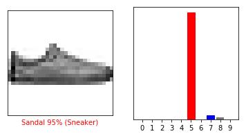
绘制多个预测结果。可以注意到,模型预测的值好高,但是依然会出错。
num_rows = 5num_cols = 3num_images = num_rows*num_colsplt.figure(figsize=(2*2*num_cols, 2*num_rows))for i in range(num_images): plt.subplot(num_rows, 2*num_cols, 2*i+1) plot_image(i, predictions[i], test_labels, test_images) plt.subplot(num_rows, 2*num_cols, 2*i+2) plot_value_array(i, predictions[i], test_labels)plt.tight_layout()plt.show()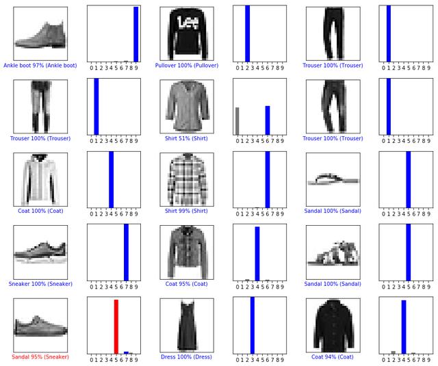
使用模型
最后,使用模型预测一个图片:
# 从测试集拿出一个样本img = test_images[1]print(img.shape)(28, 28)tf.keras模型被优化去适应 对一批数据或者一个集合进行预测。所以,如果对一个单独的样本进行预测也需要放到一个列表中。
img = (np.expand_dims(img,0))print(img.shape)(1, 28, 28)进行预测:
predictions_single = probability_model.predict(img)print(predictions_single)[[1.7000492e-04 1.5047208e-16 9.9897492e-01 1.0591678e-09 1.7027312e-04 1.2488570e-09 6.8478868e-04 1.1671354e-16 1.4649208e-13 4.2116840e-12]]plot_value_array(1, predictions_single[0], test_labels)_ = plt.xticks(range(10), class_names, rotation=45)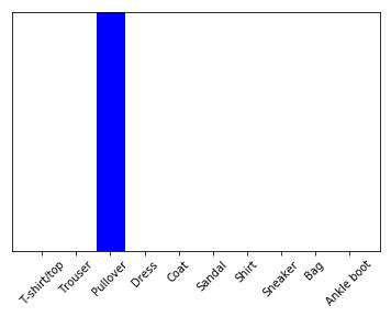
`keras.Model.predict` 返回的一个列表,其中包含被预测的样本列表的预测结果。绘制批次中唯一的图片结果:
2到此结束,希望对你有帮助~!
#TensorFlow# #深度学习# ##人工智能#


 被折叠的 条评论
为什么被折叠?
被折叠的 条评论
为什么被折叠?
 到【灌水乐园】发言


