Neural Network Week 1 & Week 2

1. Different types of neurons

• Linear neurons
• Binary threshold neurons
• Recitified linear neurons
• sigmoid neurons
• Stochastic binary neurons

 

2. Reinforcement learning

Learn to select an action to maximize payoff.

– The goal in selecting each action is to maximize the expected sum
of the future rewards.
– We usually use a discount factor for delayed rewards so that we
don’t have to look too far into the future.

Reinforcement learning is difficult:

– The rewards are typically delayed so its hard to know where we
went wrong (or right).
– A scalar reward does not supply much information.

 

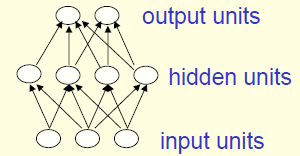
3. Main types of neural networks architecture

• Feed-forward  
  • The first layer is the input and the last layer is the output
  • They compute a series of transformations that change the similarities between cases
  • The activities of the neurons in each layer are a non-linear function of the activities in the layer below

　　

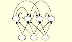
• Recurrent
  • They have directed cycles in their connection graph
  • They have complicated dynamics
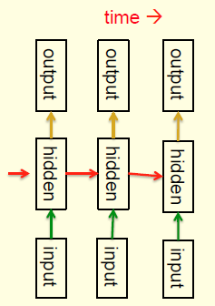
  • It is a very natural way to model sequential data
    • They are equivalent to very deep nets with one hidden layer per time slice
    • They use the same weights at every time slice and they get input at every time slice.
  • They have the ability to remember information in their hidden state

      

     

• Symmetrically connected networks
  • They are like recurrent networks but the connections between units are symmetrical(same weights in both directions)

 

4. Perceptrons

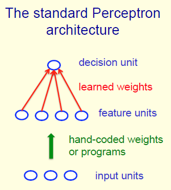
• Add an extra component with value 1 to each input vector. The “bias” weight on this component is minus the threshold. Now we can forget the threshold.

• Pick training cases using any policy that ensures that every training case willkeep getting picked.
  • If the output unit is correct, leave its weights alone
  • If the output unit incorrectly outputs a 1, subtract the input vector from the weight vector
    
  • If the output unit incorrectly outputs a zero, add the input vector to the weight vector.
•  This is guaranteed to find a set of weights that gets the right answer for all the
  training cases if any such set exists.

 

5. The limitations of Perceptrons

• once the hand-coded features have been determined, there are very strong limitations on what a perceptron can learn

• the part of a Perceptron that learns cannot learn to do this if the transformations form a group

 

转载于:https://www.cnblogs.com/climberclimb/p/7096778.html