Machine learning with python - Linear Regression

Machine learning with python

Linear Regression

              数据来自 cs229  Problem Set 1 (pdf) Data: q1x.dat, q1y.dat, q2x.dat, q2y.dat PS1 Solution (pdf)

 

 

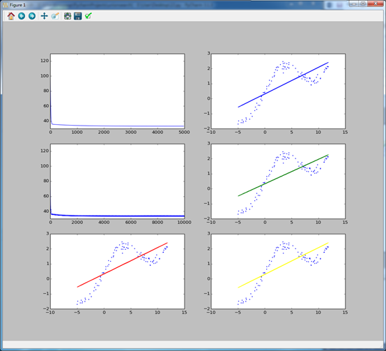
从左上往右下

batchGradientDescent的cost随迭代次数的增加而下降，和收敛结果

stochasticGradientDescent的cost随迭代次数的增加而下降，和收敛结果

normalEquations结果，ridgeRegression结果

 

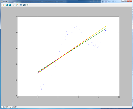
全家福，效果几乎一样

 

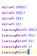
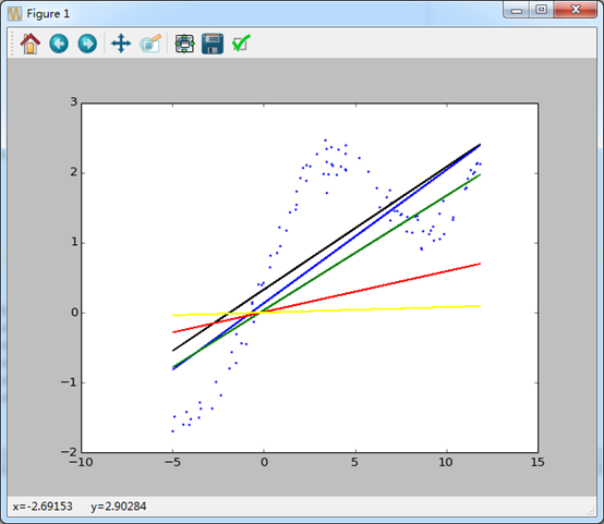
学习速率和精度对梯度下降算法的影响

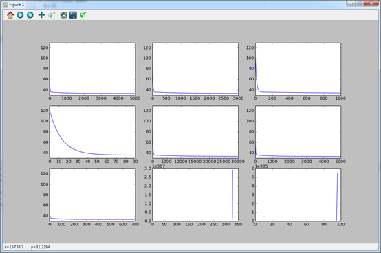
从左上往右下

最后两张略喜感，不要笑，我初始用的是1。。。花了很长时间debug

学习速率太大后果很严重

 

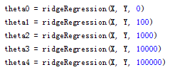
对岭回归的影响

碎碎念

为了全部矩阵化，花了不少时间

Matplotlib中文有问题，需要研究一下

不能这样表示theta -= learningRate * partialDerivativeFunc(theta, X, Y)

代码

 

 1 # !/usr/bin/python
 2 # -*- coding: utf-8 -*-
 3 # noooop
 4 
 5 import numpy as np
 6 import matplotlib.pyplot as plt
 7 
 8 def batchGradientDescent(theta, X, Y, costFunc, partialDerivativeFunc, delta=0.00001, maxIterations=100000, learningRate=0.001):
 9     cost = [costFunc(theta, X, Y), ]
10     for i in xrange(maxIterations):
11         theta = theta - learningRate * partialDerivativeFunc(theta, X, Y)
12         cost.append(costFunc(theta, X, Y))
13         if abs(cost[-1] - cost[-2]) < delta: break
14 
15     return theta, cost
16 
17 def stochasticGradientDescent(theta, X, Y,costFunc, partialDerivativeFunc, maxIterations=100, learningRate=0.001):
18     m = len(Y)
19     cost = [costFunc(theta, X, Y), ]
20     for i in xrange(maxIterations):
21         for j in xrange(m):
22             theta = theta - learningRate *partialDerivativeFunc(theta, X[j], Y[j])
23             cost.append(costFunc(theta, X, Y))
24     return theta, cost
25 
26 def normalEquations(X, Y):
27     return np.linalg.pinv(X.T.dot(X)).dot(X.T).dot(Y)
28 
29 def ridgeRegression(X, Y, lamda = 5):
30     return np.linalg.pinv(X.T.dot(X) + lamda * np.eye(2)).dot(X.T).dot(Y)
31 
32 
33 
34 def linearRegressionHypothesis(theta, X):
35     return theta.dot(X.T).T
36 
37 
38 def linearRegressionCostFunc(theta, X, Y):
39     return 0.5 * np.sum(np.array(linearRegressionHypothesis(theta, X) - Y) ** 2)
40 
41 def linearRegressionPartialDerivativeFunc(theta, X, Y):
42     return (X.T.dot(linearRegressionHypothesis(theta, X) - Y) / len(Y)).T
43 
44 def loadData(xdata, ydata):  
45     X = []  
46     Y = []
47     data = open(xdata)  
48     for line in data.readlines():  
49         X.append((1, float(line.strip())))
50     data = open(ydata) 
51     for line in data.readlines():  
52         Y.append(float(line.strip()))
53     return np.mat(X), np.mat(Y).T
54 
55 if __name__ == "__main__":
56     X, Y = loadData('q2x.dat', 'q2y.dat')
57 
58     theta0, cost0 = batchGradientDescent(np.array([[0, 0]]), X, Y, linearRegressionCostFunc, linearRegressionPartialDerivativeFunc)
59     theta1, cost1 = stochasticGradientDescent(np.array([[0, 0]]), X, Y, linearRegressionCostFunc, linearRegressionPartialDerivativeFunc)
60 
61     theta2 = normalEquations(X, Y)
62     theta3 = ridgeRegression(X, Y)
63 
64 
65     f1 = plt.figure(1)
66     #f1
67 
68     plt.subplot(321)
69     plt.plot(range(len(cost0)), cost0)
70     plt.subplot(322)
71     plt.scatter(np.array(X[:,1]),np.array(Y),color='blue',s=5,edgecolor='none')
72     plt.plot(np.array(X[:,1]),theta0[0,0] + theta0[0,1] * np.array(X[:,1]),color='blue')
73 
74     plt.subplot(323)
75     plt.plot(range(len(cost1)), cost1)
76     plt.subplot(324)
77     plt.scatter(np.array(X[:,1]),np.array(Y),color='blue',s=5,edgecolor='none')
78     plt.plot(np.array(X[:,1]),theta1[0,0] + theta1[0,1] * np.array(X[:,1]),color='green')
79 
80     plt.subplot(325)
81     plt.scatter(np.array(X[:,1]),np.array(Y),color='blue',s=5,edgecolor='none')
82     plt.plot(np.array(X[:,1]),float(theta2[0]) + float(theta2[1]) * np.array(X[:,1]),color='red')
83 
84     plt.subplot(326)
85     plt.scatter(np.array(X[:,1]),np.array(Y),color='blue',s=5,edgecolor='none')
86     plt.plot(np.array(X[:,1]),float(theta3[0]) + float(theta3[1]) * np.array(X[:,1]),color='yellow')
87 
88     f2 = plt.figure(2)
89     plt.scatter(np.array(X[:,1]),np.array(Y),color='blue',s=5,edgecolor='none')
90     plot1 = plt.plot(np.array(X[:,1]),theta0[0,0] + theta0[0,1] * np.array(X[:,1]),color='blue')
91     plot2 = plt.plot(np.array(X[:,1]),theta1[0,0] + theta1[0,1] * np.array(X[:,1]),color='green')
92     plot3 = plt.plot(np.array(X[:,1]),float(theta2[0]) + float(theta2[1]) * np.array(X[:,1]),color='red')
93     plot4 = plt.plot(np.array(X[:,1]),float(theta3[0]) + float(theta3[1]) * np.array(X[:,1]),color='yellow')
94 
95     plt.show()

 

 

 

转载于:https://www.cnblogs.com/noooop/p/3734472.html