回归模型与房价预测

import pandas as pd
pd.DataFrame(boston.data)

 

from sklearn.datasets import load_boston
boston=load_boston()
boston.keys()

dict_keys(['data', 'target', 'feature_names', 'DESCR'])

0	1	2	3	4	5	6	7	8	9	10	11	12
0	0.00632	18.0	2.31	0.0	0.538	6.575	65.2	4.0900	1.0	296.0	15.3	396.90	4.98
1	0.02731	0.0	7.07	0.0	0.469	6.421	78.9	4.9671	2.0	242.0	17.8	396.90	9.14
2	0.02729	0.0	7.07	0.0	0.469	7.185	61.1	4.9671	2.0	242.0	17.8	392.83	4.03
3	0.03237	0.0	2.18	0.0	0.458	6.998	45.8	6.0622	3.0	222.0	18.7	394.63	2.94
4	0.06905	0.0	2.18	0.0	0.458	7.147	54.2	6.0622	3.0	222.0	18.7	396.90	5.33
5	0.02985	0.0	2.18	0.0	0.458	6.430	58.7	6.0622	3.0	222.0	18.7	394.12	5.21
6	0.08829	12.5	7.87	0.0	0.524	6.012	66.6	5.5605	5.0	311.0	15.2	395.60	12.43
7	0.14455	12.5	7.87	0.0	0.524	6.172	96.1	5.9505	5.0	311.0	15.2	396.90	19.15
8	0.21124	12.5	7.87	0.0	0.524	5.631	100.0	6.0821	5.0	311.0	15.2	386.63	29.93
9	0.17004	12.5	7.87	0.0	0.524	6.004	85.9	6.5921	5.0	311.0	15.2	386.71	17.10
10	0.22489	12.5	7.87	0.0	0.524	6.377	94.3	6.3467	5.0	311.0	15.2	392.52	20.45
11	0.11747	12.5	7.87	0.0	0.524	6.009	82.9	6.2267	5.0	311.0	15.2	396.90	13.27
12	0.09378	12.5	7.87	0.0	0.524	5.889	39.0	5.4509	5.0	311.0	15.2	390.50	15.71
13	0.62976	0.0	8.14	0.0	0.538	5.949	61.8	4.7075	4.0	307.0	21.0	396.90	8.26
14	0.63796	0.0	8.14	0.0	0.538	6.096	84.5	4.4619	4.0	307.0	21.0	380.02	10.26
15	0.62739	0.0	8.14	0.0	0.538	5.834	56.5	4.4986	4.0	307.0	21.0	395.62	8.47
16	1.05393	0.0	8.14	0.0	0.538	5.935	29.3	4.4986	4.0	307.0	21.0	386.85	6.58
17	0.78420	0.0	8.14	0.0	0.538	5.990	81.7	4.2579	4.0	307.0	21.0	386.75	14.67
18	0.80271	0.0	8.14	0.0	0.538	5.456	36.6	3.7965	4.0	307.0	21.0	288.99	11.69
19	0.72580	0.0	8.14	0.0	0.538	5.727	69.5	3.7965	4.0	307.0	21.0	390.95	11.28
20	1.25179	0.0	8.14	0.0	0.538	5.570	98.1	3.7979	4.0	307.0	21.0	376.57	21.02
21	0.85204	0.0	8.14	0.0	0.538	5.965	89.2	4.0123	4.0	307.0	21.0	392.53	13.83
22	1.23247	0.0	8.14	0.0	0.538	6.142	91.7	3.9769	4.0	307.0	21.0	396.90	18.72
23	0.98843	0.0	8.14	0.0	0.538	5.813	100.0	4.0952	4.0	307.0	21.0	394.54	19.88
24	0.75026	0.0	8.14	0.0	0.538	5.924	94.1	4.3996	4.0	307.0	21.0	394.33	16.30
25	0.84054	0.0	8.14	0.0	0.538	5.599	85.7	4.4546	4.0	307.0	21.0	303.42	16.51
26	0.67191	0.0	8.14	0.0	0.538	5.813	90.3	4.6820	4.0	307.0	21.0	376.88	14.81
27	0.95577	0.0	8.14	0.0	0.538	6.047	88.8	4.4534	4.0	307.0	21.0	306.38	17.28
28	0.77299	0.0	8.14	0.0	0.538	6.495	94.4	4.4547	4.0	307.0	21.0	387.94	12.80
29	1.00245	0.0	8.14	0.0	0.538	6.674	87.3	4.2390	4.0	307.0	21.0	380.23	11.98
...	...	...	...	...	...	...	...	...	...	...	...	...	...
476	4.87141	0.0	18.10	0.0	0.614	6.484	93.6	2.3053	24.0	666.0	20.2	396.21	18.68
477	15.02340	0.0	18.10	0.0	0.614	5.304	97.3	2.1007	24.0	666.0	20.2	349.48	24.91
478	10.23300	0.0	18.10	0.0	0.614	6.185	96.7	2.1705	24.0	666.0	20.2	379.70	18.03
479	14.33370	0.0	18.10	0.0	0.614	6.229	88.0	1.9512	24.0	666.0	20.2	383.32	13.11
480	5.82401	0.0	18.10	0.0	0.532	6.242	64.7	3.4242	24.0	666.0	20.2	396.90	10.74
481	5.70818	0.0	18.10	0.0	0.532	6.750	74.9	3.3317	24.0	666.0	20.2	393.07	7.74
482	5.73116	0.0	18.10	0.0	0.532	7.061	77.0	3.4106	24.0	666.0	20.2	395.28	7.01
483	2.81838	0.0	18.10	0.0	0.532	5.762	40.3	4.0983	24.0	666.0	20.2	392.92	10.42
484	2.37857	0.0	18.10	0.0	0.583	5.871	41.9	3.7240	24.0	666.0	20.2	370.73	13.34
485	3.67367	0.0	18.10	0.0	0.583	6.312	51.9	3.9917	24.0	666.0	20.2	388.62	10.58
486	5.69175	0.0	18.10	0.0	0.583	6.114	79.8	3.5459	24.0	666.0	20.2	392.68	14.98
487	4.83567	0.0	18.10	0.0	0.583	5.905	53.2	3.1523	24.0	666.0	20.2	388.22	11.45
488	0.15086	0.0	27.74	0.0	0.609	5.454	92.7	1.8209	4.0	711.0	20.1	395.09	18.06
489	0.18337	0.0	27.74	0.0	0.609	5.414	98.3	1.7554	4.0	711.0	20.1	344.05	23.97
490	0.20746	0.0	27.74	0.0	0.609	5.093	98.0	1.8226	4.0	711.0	20.1	318.43	29.68
491	0.10574	0.0	27.74	0.0	0.609	5.983	98.8	1.8681	4.0	711.0	20.1	390.11	18.07
492	0.11132	0.0	27.74	0.0	0.609	5.983	83.5	2.1099	4.0	711.0	20.1	396.90	13.35
493	0.17331	0.0	9.69	0.0	0.585	5.707	54.0	2.3817	6.0	391.0	19.2	396.90	12.01
494	0.27957	0.0	9.69	0.0	0.585	5.926	42.6	2.3817	6.0	391.0	19.2	396.90	13.59
495	0.17899	0.0	9.69	0.0	0.585	5.670	28.8	2.7986	6.0	391.0	19.2	393.29	17.60
496	0.28960	0.0	9.69	0.0	0.585	5.390	72.9	2.7986	6.0	391.0	19.2	396.90	21.14
497	0.26838	0.0	9.69	0.0	0.585	5.794	70.6	2.8927	6.0	391.0	19.2	396.90	14.10
498	0.23912	0.0	9.69	0.0	0.585	6.019	65.3	2.4091	6.0	391.0	19.2	396.90	12.92
499	0.17783	0.0	9.69	0.0	0.585	5.569	73.5	2.3999	6.0	391.0	19.2	395.77	15.10
500	0.22438	0.0	9.69	0.0	0.585	6.027	79.7	2.4982	6.0	391.0	19.2	396.90	14.33
501	0.06263	0.0	11.93	0.0	0.573	6.593	69.1	2.4786	1.0	273.0	21.0	391.99	9.67
502	0.04527	0.0	11.93	0.0	0.573	6.120	76.7	2.2875	1.0	273.0	21.0	396.90	9.08
503	0.06076	0.0	11.93	0.0	0.573	6.976	91.0	2.1675	1.0	273.0	21.0	396.90	5.64
504	0.10959	0.0	11.93	0.0	0.573	6.794	89.3	2.3889	1.0	273.0	21.0	393.45	6.48
505	0.04741	0.0	11.93	0.0	0.573	6.030	80.8	2.5050	1.0	273.0	21.0	396.90	7.88

506 rows × 13 columns

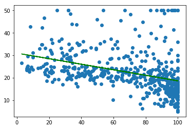
data=boston.data
x=data[:,6]
y=boston.target

from sklearn.linear_model import LinearRegression
LineR=LinearRegression()
LineR.fit(x.reshape(-1,1),y)
w=LineR.coef_
b=LineR.intercept_
print(w,b)

import matplotlib.pyplot as pl
pl.scatter(x,y)
pl.plot(x,w*x+b,'g')
pl.show()

 

[-0.12316272] 30.97867776261804

 

 

 

 

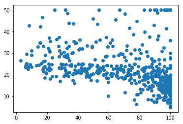
xx=data[:,6].reshape(-1,1)
pl.scatter(xx,y)
pl.show()

from sklearn.preprocessing import PolynomialFeatures
p=PolynomialFeatures()
p.fit(xx)
p.transform(xx)

 

Out[51]:

array([[1.00000e+00, 6.52000e+01, 4.25104e+03],
       [1.00000e+00, 7.89000e+01, 6.22521e+03],
       [1.00000e+00, 6.11000e+01, 3.73321e+03],
       ...,
       [1.00000e+00, 9.10000e+01, 8.28100e+03],
       [1.00000e+00, 8.93000e+01, 7.97449e+03],
       [1.00000e+00, 8.08000e+01, 6.52864e+03]])

x_poly=p.transform(xx)
x_poly

lrp=LinearRegression()
lrp.fit(x_poly,y)
y_poly=lrp.predict(x_poly)
pl.scatter(xx,y)
pl.plot(xx,w*xx+b,'r')
pl.scatter(xx,y_poly)
pl.show()
lrp.coef_

 

 

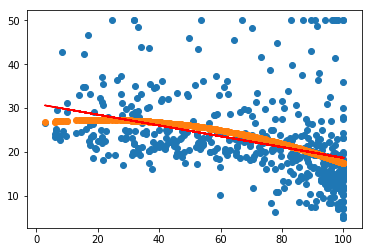
array([ 0.        ,  0.06919309, -0.00159822])

转载于:https://www.cnblogs.com/lbjdaxiong/p/10095547.html