Chi-Square test in R

Chi-Square

Chi-Square distribution test

This Chi-Square test is used to assess fitting

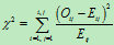
Chi-Squared value is:

: is the observed value of class i

: is the expected value of class i

if is close to , is 0, could be an indicator shows the close level of observed distribution to the expected distribution. Normal distribution is a special case.

 

Chi-Square test also could be used to assess the fitting.

Example:

> O <- c(21,42,24,8,4,1) # Suppose we have a observed values

> N <- sum(E) # the sample size

> N

[1] 100

> c1 <- pbinom(0,5,.25) # Guess the sample should have The Binomial Distribution find it's expected probability

> c2 <- pbinom(1,5,.25)-pbinom(0,5,.25)

> c3 <- pbinom(2,5,.25)-pbinom(1,5,.25)

> c4 <- pbinom(3,5,.25)-pbinom(2,5,.25)

> c5 <- pbinom(4,5,.25)-pbinom(3,5,.25)

> c6 <- pbinom(5,5,.25)-pbinom(4,5,.25)

> P <- c(c1,c2,c3,c4,c5,c6)

> P

[1] 0.2373046875 0.3955078125 0.2636718750

[4] 0.0878906250 0.0146484375 0.0009765625

> sum(P)

[1] 1

> E <- P*N # calculate the expected frequency value in 100 samples

> E

[1] 23.73046875 39.55078125 26.36718750

[4] 8.78906250 1.46484375 0.09765625

> sum((O-E)^2/E) # calculate the chi-square value

[1] 13.47437

> 1-pchisq(13.47437,5) # calculate the p-value

[1] 0.01931663

p-value < 0.05

 

The goodness for fitting assess rules (you could set your own rules for your data):

p-value >= 0.25 Excellent fit

0.15 =< p-value < 0.25 Good fit

0.05 =< p-value < 0.15 Moderately Good fit

0.01 =< p-value < 0.05 Poor fit

 

Reject the null hypothesis, since we don't have significant evidence which indicate the E is Binomial Distribution.

 

Chi-Square Test for Independence

This lesson explains how to conduct a chi-square test for independence. The test is applied when you have two categorical variables from a single population. It is used to determine whether there is a significant association between the two variables.

For example, in an election survey, voters might be classified by gender (male or female) and voting preference (Democrat, Republican, or Independent). We could use a chi-square test for independence to determine whether gender is related to voting preference. The sample problem at the end of the lesson considers this example.

The test procedure described in this lesson is appropriate when the following conditions are met:

1. The sampling method is simple random sampling.
2. Each population is at least 10 times as large as its respective sample.
3. The variables under study are each categorical.
4. If sample data are displayed in a contingency table, the expected frequency count for each cell of the table is at least 5.

This approach consists of four steps: (1) state the hypotheses, (2) formulate an analysis plan, (3) analyze sample data, and (4) interpret results.

 

We set variable x and variable y as two categories, and test the independence of x and y. contain x and y in the same Contingency Table, the row is categories of x and the column is the categories of y.

	X1	X2	X3
Y1	O11	O12	O13
Y2	O21	O22	O23
Y3	O31	O32	O33

calculate the total number of each row and column show the table below:

	X1	X2	X3	Total in row
Y1	O11	O12	O13	Oy1=O11+ O12+ O13
Y2	O21	O22	O23	Oy2=O21+ O22+ O23
Y3	O31	O32	O33	Oy3=O31+ O32+ O33
Total in column	Ox1=O11+ O21+ O31	Ox2=O12+ O22+ O32	Ox3=O13+ O23+ O33	sample size N

 

Formula:

where O represents the observed frequency. E is the expected frequency under the null hypothesis and computed by

Example:

 

> library(MASS)

> tbl = table(survey$Smoke, survey$Exer)

> tb1

Error: object 'tb1' not found

> tbl

 

Freq None Some

Heavy 7 1 3

Never 87 18 84

Occas 12 3 4

Regul 9 1 7

 

The Smoke column records the students smoking habit, while the Exer column records their exercise level. The allowed values in Smoke are "Heavy", "Regul" (regularly), "Occas" (occasionally) and "Never". As for Exer, they are "Freq" (frequently), "Some" and "None".

test if Exer and Smoke are independent.

> chisq.test(tbl)

Result:

    Pearson's Chi-squared test

 

data: tbl

X-squared = 5.4885, df = 6, p-value = 0.4828

Set the significance value is 0.05, p-value>0.05, we do not reject the null hypothesis that the smoking habit is independent of the exercise level of the students.

 

null hypothesis: the variables are independent.

alternative hypothesis: the variables are not independent.

 

 

Reference:

http://dist.stat.tamu.edu/pub/rvideos/Chi-Square2/Chi-Square.html

Weisstein, Eric W. "Chi-Squared Distribution." From MathWorld--A Wolfram Web Resource. http://mathworld.wolfram.com/Chi-SquaredDistribution.html

http://stattrek.com/chi-square-test/independence.aspx

https://onlinecourses.science.psu.edu/stat500/node/56

转载于:https://www.cnblogs.com/chaseskyline/p/3786048.html