深度学习噪声抑制_使用深度学习抑制噪声-优快云博客

本文探讨了如何利用深度学习进行噪声抑制，介绍了相关的方法和应用，旨在提升语音和音频信号的质量。

摘要生成于 C知道，由 DeepSeek-R1 满血版支持，前往体验 >

深度学习噪声抑制

At the time of boom of online video conferencing and virtual communication, the ability of a platform to suppress background noise plays a crucial roll to give it a leading edge. Platforms like Google Meet constantly use Machine Learning to perform noise suppression to provide the best audio quality possible. Today I will show you how you could make your own Deep Learning model to perform Noise Suppression

在在线视频会议和虚拟通信蓬勃发展之际，平台抑制背景噪声的能力发挥了至关重要的作用，从而使其具有领先优势。像Google Meet这样的平台不断使用机器学习来执行噪声抑制，以提供最佳的音频质量。今天，我将向您展示如何创建自己的深度学习模型来执行噪声抑制

抑制噪音有什么大不了的？(What’s the Big Deal with Noise Suppression?)

The task of Noise Suppression can be approached in a few different ways. These might include Generative Adversarial Networks (GAN’s), Embedding Based Models, Residual Networks, etc. Irrespective of the approach, there are two major problems with Noise Suppression

噪声抑制的任务可以通过几种不同的方法来解决。这些可能包括生成对抗网络(GAN)，基于嵌入的模型，残差网络等。不管采用哪种方法，噪声抑制都有两个主要问题

Handling variable length audio sequences
处理可变长度的音频序列
Slow processing time resulting in lag
缓慢的处理时间导致滞后

I will show you some basic methods in this article on how to deal with these problems

我将在本文中向您展示一些有关如何解决这些问题的基本方法

开始吧(Let’s Start)

We will first import our libraries. We will be using tensorflow. You are free to implement a PyTorch version of the same.

我们将首先导入我们的库。我们将使用tensorflow。您可以自由地实现相同的PyTorch版本。

import tensorflow as tf
from tensorflow.keras.layers import Conv1D,Conv1DTranspose,Concatenate,Input
import numpy as np
import IPython.display
import glob
from tqdm.notebook import tqdm
import librosa.display
import matplotlib.pyplot as plt

The data we will be using is a combination of Clean and Noisy audio samples of different sizes. The dataset is provided by University of Edinburgh and can be downloaded from here

我们将使用的数据是不同大小的Clean和Noisy音频样本的组合。数据集由爱丁堡大学提供，可从此处下载

加载和可视化数据(Loading and Visualising the data)

We will use tensorflow’s tf.audio module to load our data. Using tf.audio() along with tf.io.read_file() has given me 50% faster loading times as compared to librosa.load() because of tensorflow using the GPU

我们将使用tensorflow的tf.audio模块加载我们的数据。与librosa.load()相比，将tf.audio()与tf.io.read_file()结合使用可使我的加载时间缩短了50％，这是因为使用GPU进行了张量流

clean_sounds = glob.glob('/content/CleanData/*')
noisy_sounds = glob.glob('/content/NoisyData/*')


clean_sounds_list,_ = tf.audio.decode_wav(tf.io.read_file(clean_sounds[0]),desired_channels=1)
for i in tqdm(clean_sounds[1:]):
  so,_ = tf.audio.decode_wav(tf.io.read_file(i),desired_channels=1)
  clean_sounds_list = tf.concat((clean_sounds_list,so),0)


noisy_sounds_list,_ = tf.audio.decode_wav(tf.io.read_file(noisy_sounds[0]),desired_channels=1)
for i in tqdm(noisy_sounds[1:]):
  so,_ = tf.audio.decode_wav(tf.io.read_file(i),desired_channels=1)
  noisy_sounds_list = tf.concat((noisy_sounds_list,so),0)


clean_sounds_list.shape,noisy_sounds_list.shape

Here we load our individual audio files using tf.audio.decode_wav() and concatentate them to get two tensors named clean_sounds_list and noisy_sounds_list. This process takes about 3–4 minutes to complete and is visually represented using the tqdm loading bar

在这里，我们使用tf.audio.decode_wav()加载我们的单个音频文件，并使其合并以获得两个名为clean_sounds_list和noisy_sounds_list的张量。此过程大约需要3-4分钟才能完成，并使用tqdm加载栏直观地表示出来

batching_size = 12000


clean_train,noisy_train = [],[]


for i in tqdm(range(0,clean_sounds_list.shape[0]-batching_size,batching_size)):
  clean_train.append(clean_sounds_list[i:i+batching_size])
  noisy_train.append(noisy_sounds_list[i:i+batching_size])


clean_train = tf.stack(clean_train)
noisy_train = tf.stack(noisy_train)


clean_train.shape,noisy_train.shape

After the loading is done, we will need to make uniform splits of the one big audio waveform. Although this is not compulsory to do, our main aim is to convert this model to a tflite model which currently, does not support variable length inputs. I decided an arbitrary value of batching_size as 12000. You are free to change it but keep it as small as possible. It will be useful later.

加载完成后，我们将需要对一个大音频波形进行均匀分割。尽管这不是强制性的，但我们的主要目标是将该模型转换为tflite模型，该模型目前不支持可变长度输入。我决定将batching_size的任意值设置为12000。您可以随意更改它，但请使其尽可能小。以后会有用。

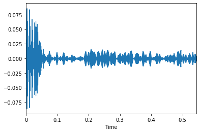
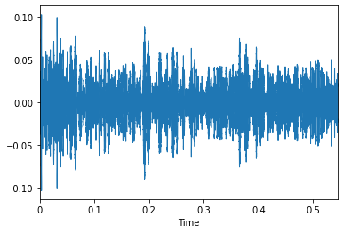
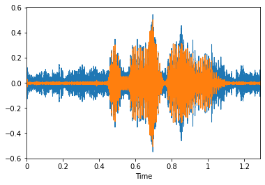
For the visualising part, we use librosa’s display module which basically uses matplotlib in the backend to plot the data. On plotting the data as seen above, we can see that the noise is quite visible. The noise can be anything ranging from people and cars to dish-washing sounds.

对于可视化部分，我们使用librosa的显示模块，该模块基本上在后端使用matplotlib绘制数据。如上所示，在绘制数据时，我们可以看到噪声非常明显。噪音可以是从人和汽车到洗碗碟声音的任何东西。

创建用于流水线的tf.data.Dataset (Creating a tf.data.Dataset for pipelining)

We will now create a very basic helper function called get_dataset() to generate a tf.data.Dataset. We choose 40000 samples for training and the remaining 5000 for testing. Again, you are free to tweak and add to this but I will not be going into the depth here as pipeline optimization is not the main goal of this article

现在，我们将创建一个非常基本的辅助函数，称为get_dataset()来生成tf.data.Dataset。我们选择40000个样本进行训练，其余5000个样本进行测试。同样，您可以随意调整并添加此内容，但由于管道优化不是本文的主要目标，因此我不会在此深入探讨

def get_dataset(x_train,y_train):
  dataset = tf.data.Dataset.from_tensor_slices((x_train,y_train))
  dataset = dataset.shuffle(100).batch(64,drop_remainder=True)
  return dataset
  
train_dataset = get_dataset(noisy_train[:40000],clean_train[:40000])
test_dataset = get_dataset(noisy_train[40000:],clean_train[40000:])

创建模型(Creating the Model)

The code for the model architecture is as follows:

模型架构的代码如下：

inp = Input(shape=(batching_size,1))
c1 = Conv1D(2,32,2,'same',activation='relu')(inp)
c2 = Conv1D(4,32,2,'same',activation='relu')(c1)
c3 = Conv1D(8,32,2,'same',activation='relu')(c2)
c4 = Conv1D(16,32,2,'same',activation='relu')(c3)
c5 = Conv1D(32,32,2,'same',activation='relu')(c4)


dc1 = Conv1DTranspose(32,32,1,padding='same')(c5)
conc = Concatenate()([c5,dc1])
dc2 = Conv1DTranspose(16,32,2,padding='same')(conc)
conc = Concatenate()([c4,dc2])
dc3 = Conv1DTranspose(8,32,2,padding='same')(conc)
conc = Concatenate()([c3,dc3])
dc4 = Conv1DTranspose(4,32,2,padding='same')(conc)
conc = Concatenate()([c2,dc4])
dc5 = Conv1DTranspose(2,32,2,padding='same')(conc)
conc = Concatenate()([c1,dc5])
dc6 = Conv1DTranspose(1,32,2,padding='same')(conc)
conc = Concatenate()([inp,dc6])
dc7 = Conv1DTranspose(1,32,1,padding='same',activation='linear')(conc)
model = tf.keras.models.Model(inp,dc7)
model.summary()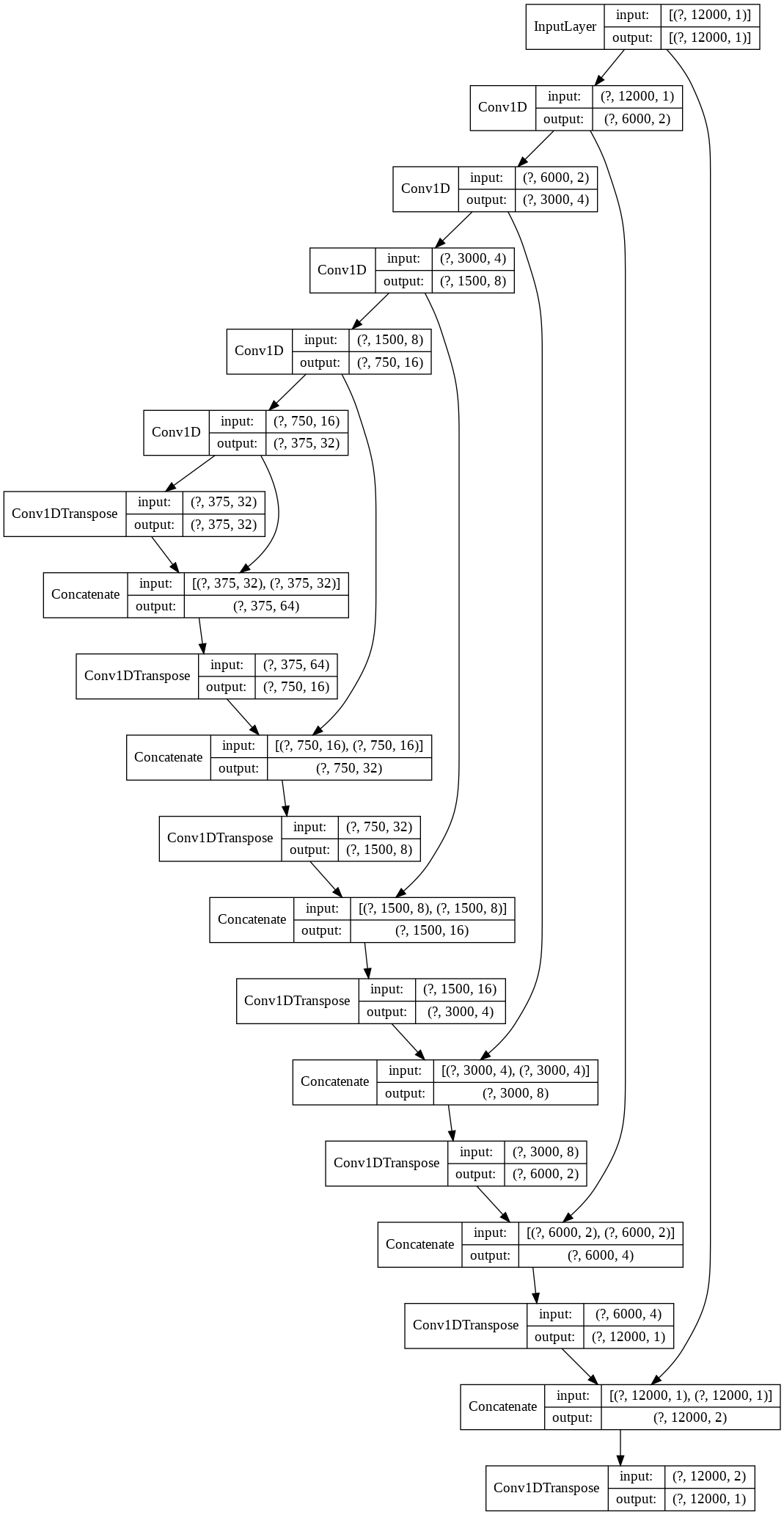

The model is a purely Convolutional one. The goal is to find a bunch of filters so as to help minimize the background noise. To help with this, we add residual connections to help with context from the original audio sample. The idea behind this model is derived from the implementation of SEGAN network [et.al Santiago Pascual]. The idea derives from the fact that a purely convolutional network can handle multiple shape inputs with ease, leading to more flexibility. The convolutional nature forces the model to focus on the temporally close correlations throughout the model. The model can be split into two parts, the convolutions and the de-convolutions(or upsampling layers). The strided convolutional layers behave as an auto-encoder where after N layers, a reduced representation of the input is obtained. The deconvolutions perform exactly the opposite strided procedures to obtain a cleaned representation of the noisy input. The skip connections provide the required context to the deconvolution layers at every step which results in better overall results.

该模型是纯粹的卷积模型。目标是找到一堆滤波器，以帮助最小化背景噪声。为了解决这个问题，我们添加了残余连接以帮助处理原始音频样本中的上下文。该模型背后的思想源自SEGAN网络的实施[et.al Santiago Pascual ]。该思想源于以下事实：纯卷积网络可以轻松处理多种形状输入，从而带来更大的灵活性。卷积性质迫使模型将注意力集中在整个模型的时间紧密相关性上。该模型可以分为两部分：卷积和反卷积(或上采样层)。跨步的卷积层表现为自动编码器，其中在N层之后，获得了输入的简化表示。解卷积执行完全相反的跨步过程，以获得带噪输入的清晰表示。跳过连接在每个步骤都为反卷积层提供了所需的上下文，从而带来了更好的总体效果。

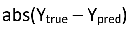
The model is compiled with a Mean Absolute Loss

使用平均绝对损失编译模型

The choice of optimizer was difficult as, SGD,RMSprop and Adam stood pretty close. I finally went ahead with Adam just because of it’s slightly more robust nature. Some hyperparameter tweaking gave me a pretty good learning rate of 0.002

由于SGD，RMSprop和Adam处于非常接近的位置，因此很难选择优化器。我最终还是选择了Adam，只是因为它的特性更加强大。一些超参数调整使我的学习率达到了0.002

The final results:

最终结果：

Training loss: 0.0117
训练损失：0.0117
Testing loss: 0.0117
测试损失：0.0117

The results are quite pleasing but we are not done yet. We still have to handle the inference procedure for variable sized inputs. We will do that next

结果非常令人满意，但我们尚未完成。对于可变大小的输入，我们仍然必须处理推理过程。接下来我们会做

处理可变输入形状(Handling the Variable Input Shape)

Our model is trained with a very specific input shape which is dependent on our batching_size. To allow multiple shape inputs, a simple strategy will work really well.

我们的模型使用非常具体的输入形状进行训练，具体取决于我们的batching_size。 为了允许多种形状输入，一种简单的策略将非常有效。

We run our model through all the splits till the (n-1)th split. Consider the example where batching_size is 12000 and your audio array is of shape (37500,). In this case we split the audio waveform into min(37500/12000) = 3 splits. The remaining part of the array will be of shape (1500,). To fix this problem we sample another frame but this time from the rear end of the array. Something like this

我们通过所有拆分运行模型，直到第(n-1)个拆分为止。考虑以下示例，其中batching_size为12000，并且音频阵列的形状为(37500，)。在这种情况下，我们将音频波形分割为min(37500/12000)= 3分割。数组的其余部分将具有形状(1500，)。为了解决这个问题，我们从阵列的后端取样另一个帧，但这一次。像这样

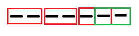
Now, we run all the 4 splits through the model to get individual predictions.
现在，我们对模型进行所有4个拆分，以获取单独的预测。
From the output predictions, we extract the first three frames as they are and clip the last frame to get only the remaining part
从输出预测中，我们按原样提取前三个帧，然后裁剪最后一帧以仅获取剩余部分

At this point, some code will help with clarity

在这一点上，一些代码将有助于澄清

def get_audio(path):
  audio,_ = tf.audio.decode_wav(tf.io.read_file(path),1)
  return audio


def inference_preprocess(path):
  audio = get_audio(path)
  audio_len = audio.shape[0]
  batches = []
  for i in range(0,audio_len-batching_size,batching_size):
    batches.append(audio[i:i+batching_size])


  batches.append(audio[-batching_size:])
  diff = audio_len - (i + batching_size)  # Calculation of length of remaining waveform
  return tf.stack(batches), diff


def predict(path):
  test_data,diff = inference_preprocess(path)
  predictions = model.predict(test_data)
  final_op = tf.reshape(predictions[:-1],((predictions.shape[0]-1)*predictions.shape[1],1))  # Reshape the array to get complete frames
  final_op = tf.concat((final_op,predictions[-1][-diff:]),axis=0)  # Concat last, incomplete frame to the rest
  return final_op

好吧，那有多快？(Okay but how fast is it?)

%%timeit
 tf.squeeze(predict(noisy_sounds[3]))OUTPUT: 10 loops, best of 3: 31.3 ms per loop

If we specify the input shape of the model as (None,1), we can pass a variable length tensor to the model which gives even faster results. For now, we want to quantize the model for cross device compatibility.

如果我们将模型的输入形状指定为(None，1)，则可以将可变长度张量传递给模型，从而获得更快的结果。目前，我们想对模型进行量化以实现跨设备兼容性。

TFLite模型的优化和创建 (Optimization and Creation of TFLite Model)

Using the TFLiteConverter() is pretty straightforward. You pass the keras model along with an optimization strategy (TF documentation recommends using DEFAULT only) and write the converted model to a binary file for future use.

使用TFLiteConverter()非常简单。您将keras模型与优化策略(TF文档建议仅使用DEFAULT)一起传递，并将转换后的模型写入二进制文件以备将来使用。

lite_model = tf.lite.TFLiteConverter.from_keras_model(model)
lite_model.optimizations = [tf.lite.Optimize.DEFAULT]
tflite_model_quant = lite_model.convert()


with open('TFLiteModel.tflite','wb') as f:
  f.write(tflite_model_quant)

TFLite模型推论(TFLite Model Inference)

The preprocessing is similar to that of the Keras model but since I could not find anything on batching for TFLite models (please let me know if the support is present), I had to use a pythonic for loop for iterating over all splits. The code below describes instantiation of the Interpreter and allocation of tensors, followed by invoking it to get us our results

预处理与Keras模型类似，但是由于我在批处理中找不到TFLite模型的任何内容(请告诉我是否存在支持)，因此我不得不使用pythonic for循环遍历所有拆分。下面的代码描述了解释器的实例化和张量的分配，然后调用它来获得我们的结果

# Initializing the Interpreter and allocating tensors
interpreter = tf.lite.Interpreter(model_path='/content/TFLiteModel.tflite')
interpreter.allocate_tensors()


def predict_tflite(path):
  test_audio,diff = inference_preprocess(path)
  input_index = interpreter.get_input_details()[0]["index"]
  output_index = interpreter.get_output_details()[0]["index"]


  preds = []
  for i in test_audio:
    interpreter.set_tensor(input_index, tf.expand_dims(i,0))  # We will have to pass individual splits since tflite doesn't support batching at this moment
    interpreter.invoke()
    predictions = interpreter.get_tensor(output_index)
    preds.append(predictions)


  predictions = tf.squeeze(tf.stack(preds,axis=1))
  final_op = tf.reshape(predictions[:-1],((predictions.shape[0]-1)*predictions.shape[1],1))
  final_op = tf.concat((tf.squeeze(final_op),predictions[-1][-diff:]),axis=0)
  return final_op

Now the question arises, how better is this than the Keras model? The answer to that isn’t simple. Since I was unable to to process all batches together, the overall inference time was affected but the TFLite Model on it’s own is faster than the Keras model.

现在出现了问题，这比Keras模型好吗？答案并不简单。由于我无法同时处理所有批次，因此总体推理时间受到影响，但是TFLite模型本身比Keras模型要快。

%%timeit
 predict_tflite(noisy_sounds[3])OUTPUT: 10 loops, best of 3: 41.7 ms per loop

Out of all the advantages of the TFLite format, cross platform deployment is the biggest one. The model can now be ported much easily than the Keras model, not to mention the super small size of the model- just 346 kB

在TFLite格式的所有优势中，跨平台部署是最大的优势。与Keras模型相比，该模型现在可以轻松移植，更不用说模型的超小尺寸-仅346 kB

现在就这样！(That’s it for now!)

The model can be improved further by addition of filters, creating a deeper model and optimizing the pipeline but that is for next time. As we come to the end of the article I would like to mention some references and links.

可以通过添加过滤器，创建更深的模型并优化管道来进一步改善模型，但这是下一次。当我们到本文结尾时，我想提及一些参考和链接。

Colab Notebook for the code and audio samples: Here
Colab Notebook的代码和音频示例：这里
Dataset: Here
数据集：此处
SEGAN paper: Here
SEGAN纸：在这里

Any comments or suggestions would be much appreciated. Thanks for reading!

任何意见或建议将不胜感激。谢谢阅读！

翻译自: https://medium.com/analytics-vidhya/noise-suppression-using-deep-learning-6ead8c8a1839