咖啡茶

最新推荐文章于 2025-05-23 09:16:47 发布

weixin_26729283

最新推荐文章于 2025-05-23 09:16:47 发布

阅读量384

点赞数

文章标签： python

原文链接：https://medium.com/towards-artificial-intelligence/coffee-tea-emd-19d1c387ea5e

版权

本文通过使用Empirical Mode Decomposition (EMD) 和 Fast Fourier Transform (FFT) 分析了印度咖啡与茶的价格数据，揭示了价格的趋势和周期性特征。

摘要生成于 C知道，由 DeepSeek-R1 满血版支持，前往体验 >

数据科学 (Data Science)

前言 (Preface)

My mornings usually begin with a mug of steaming black coffee. No, it’s not the expensive gourmet stuff, but the instant coffee powder that powers me through the rest of the morning.

我的早晨通常从一杯热气腾腾的黑咖啡开始。不，不是昂贵的美食，而是速溶咖啡粉在整个早晨为我提供动力。

My evenings are usually more mellow, with a nice cup of strong Indian tea and perhaps a couple of biscuits. They provide just the right amount of caffeine to make it all the way to 10 pm.

我的夜晚通常更柔和，可以喝一杯浓烈的印度茶，也可以喝几杯饼干。他们提供适量的咖啡因，使它一直持续到晚上10点。

动机 (Motivation)

I recently had to use a nifty signal processing tool — Empirical Mode Decomposition (EMD)— at work and thought this would make for an interesting post!

最近，我不得不在工作中使用一个精巧的信号处理工具- Empirical Mode Decomposition (EMD) ，并认为这将成为一篇有趣的文章！

In this article, I would be using the prices of my favorite beverages to give a high-level overview of EMD and also touch upon Fast Fourier Transform (FFT).

在本文中，我将使用我最喜欢的饮料的价格对EMD进行高级概述，同时还涉及Fast Fourier Transform (FFT) 。

These techniques are not restricted to the signal processing domain and can easily be used on any time-series data to derive extremely useful insights!

这些技术不仅限于信号处理领域，还可以轻松地用于任何时间序列数据，以获取极为有用的见解！

As always, you can check out the entire code on my GitHub repository.

与往常一样，您可以在我的 GitHub 存储库中 签出整个代码 。

数据源 (Data Source)

The open data portal hosted by the Indian Government — www.data.gov.in was a good place to search for my needs. I found some commodities datasets that seemed clean enough to work with. Some of the data was a bit outdated, but for my little exercise, I reasoned that it would be sufficient. So I ended up downloading datasets for loose tea and powdered coffee.

印度政府托管的开放数据门户网站www.data.gov.in是寻找我的需求的好地方。我发现一些商品数据集看起来足够干净可以使用。有些数据有些过时了，但是对于我的少量练习，我认为这样就足够了。因此，我最终下载了散茶和咖啡粉的数据集。

关于数据 (About the Data)

The dataset contains information on the daily wholesale prices of the commodities I mentioned. The prices were primarily the rates at which the commodity was sold in the wholesale markets.

该数据集包含有关我提到的商品的每日批发价格的信息。价格主要是商品在批发市场上的销售价格。

The dataset for the loose tea leaves looks like this —

散茶叶的数据集看起来像这样-

<class 'pandas.core.frame.DataFrame'>
DatetimeIndex: 114495 entries, 1997-11-25 to 2015-04-28
Data columns (total 3 columns):
 #   Column          Non-Null Count   Dtype  
---  ------          --------------   -----  
 0   Centre_Name     114495 non-null  object 
 1   Commodity_Name  114495 non-null  object 
 2   Price           114495 non-null  float64
dtypes: float64(1), object(2)
memory usage: 3.5+ MB

As you see the dataset is pretty limited in features, but that was fine with me, because I wanted to look at the price alone. The dataset for the powdered coffee looked like this —

如您所见，数据集的功能非常有限，但对我来说很好，因为我只想看看价格。咖啡粉的数据集看起来像这样-

<class 'pandas.core.frame.DataFrame'>
DatetimeIndex: 11515 entries, 2003-01-07 to 2019-12-02
Data columns (total 8 columns):
 #   Column       Non-Null Count  Dtype 
---  ------       --------------  ----- 
 0   state        11515 non-null  object
 1   district     11515 non-null  object
 2   market       11515 non-null  object
 3   commodity    11515 non-null  object
 4   variety      11515 non-null  object
 5   min_price    11515 non-null  int64 
 6   max_price    11515 non-null  int64 
 7   modal_price  11515 non-null  int64 
dtypes: int64(3), object(5)
memory usage: 809.6+ KB

Although this dataset was a little richer in features, I used only the modal price (most common price in a day) so as to keep things simple.

尽管此数据集的功能有些丰富，但我仅使用模式价格( 一天中最常见的价格)以使事情变得简单。

数据预处理 (Data Preprocessing)

After a little pre-processing magic,

经过一点预处理魔术之后，

# We select the modal_price for coffee and aggregate over the whole country
data0 = coffee_df.loc['2010':'2014', 'modal_price'].resample('D').mean()
# We aggregate over the whole country for the loose tea prices
data1 = tea_df.loc['2010':'2014', 'Price'].resample('D').mean()
# We concatenate the data and fill in missing values
comm_df = pd.concat([data0, data1],axis=1)
comm_df.columns = ['coffee','tea']
comm_df = comm_df.dropna()
comm_df = comm_df.fillna(method='ffill')

the data was good to go!

数据很好！

<class 'pandas.core.frame.DataFrame'>
DatetimeIndex: 1121 entries, 2010-01-01 to 2014-12-31
Data columns (total 2 columns):
 #   Column  Non-Null Count  Dtype  
---  ------  --------------  -----  
 0   coffee  1121 non-null   float64
 1   tea     1121 non-null   float64
dtypes: float64(2)
memory usage: 26.3 KB

统计摘要 (Summary Statistics)

The customary summary statistics for the dataset is given below —

数据集的常规摘要统计信息如下-

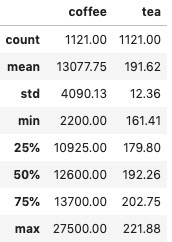
Coffee: Rupees per quintal (1 quintal = 100 kg)
咖啡：每公担卢比(1公分= 100公斤)
Loose Tea Leaves: Rupees per quintal
散茶叶：每公担的卢比

From the summary statistics, it is clear that coffee is the more expensive commodity among the two and also the one to show large fluctuation over the years. Tea is the more stable and also the cheaper option between the two beverages in India.

从汇总统计数据中可以明显看出，咖啡是两者中较昂贵的商品，并且也是多年来波动较大的商品。茶是印度两种饮料中比较稳定且便宜的选择。

时间序列分析 (Time Series Analysis)

时间序列图 (Time Series Plot)

The first thing to do is to plot the commodity prices as a time series, with the daily highs and lows enveloping it.

首先要做的是将商品价格绘制成一个时间序列，将每日的高点和低点包裹起来。

fig, ax = plt.subplots(2,1, sharex=True, figsize=[15,10])for i in range(0,2):
    c = comm_df.iloc[:,i]
    c_low = c.resample('W').min()
    c_high = c.resample('W').max()
    c_mean = c.resample('W').mean()
    ax[i].plot(c_low.index, c_low.values, linewidth=2, linestyle='')
    ax[i].plot(c_mean.index, c_mean.values, linewidth=2, color='k')
    ax[i].plot(c_high.index, c_high.values, linewidth=2, linestyle='')
    ax[i].fill_between(c_low.index, c_low.values, c_high.values, alpha=0.5)
    ax[i].set_ylabel(comm_df.columns[i])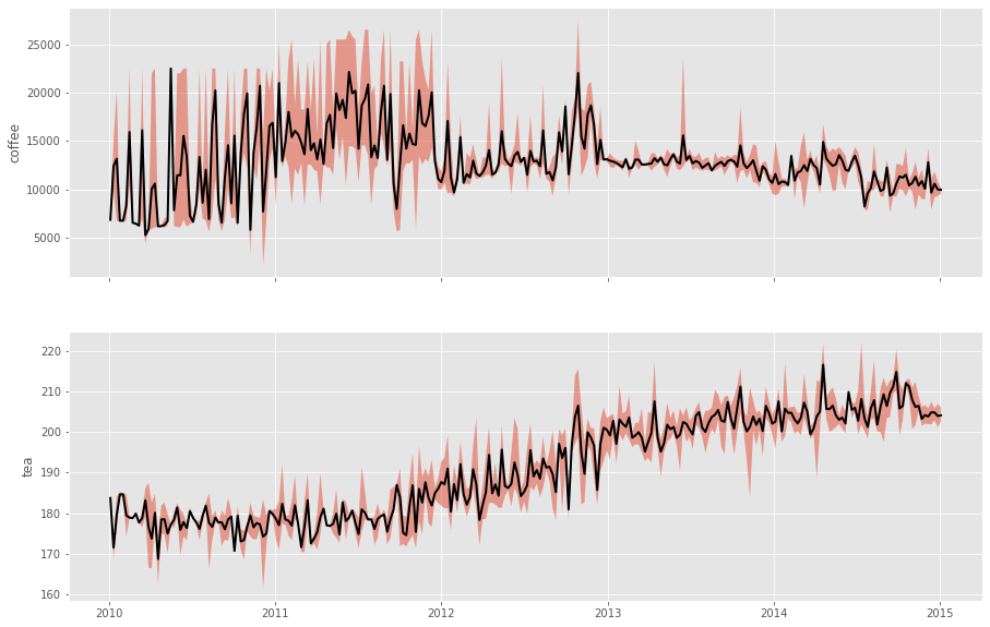

Observations:

Large fluctuations are observed in coffee prices, especially in 2011–12;
咖啡价格波动很大，尤其是在2011-12年度；
There seems to be some seasonality in the prices (or in other words, some oscillations or periodicity in the time series);
价格似乎有一些季节性( 或者说时间序列中有一些波动或周期性 )；
Tea shows a rising trend in prices, but the trend isn’t immediately obvious for Coffee.
茶的价格呈上升趋势，但对于咖啡而言，这种趋势并不立即明显。

A monthly variation plot using seaborn will give additional insight —

使用seaborn每月变化图将提供更多见解-

fig,ax = plt.subplots(1,2,figsize=[15,6])
sns.lineplot(comm_df.index.month, comm_df.coffee, color='teal', ax=ax[0])
ax[0].set_xlabel('Month')
ax[0].set_ylabel('Coffee Price (Rs/quintal)')sns.lineplot(comm_df.index.month, comm_df.tea, color='green', ax=ax[1])
ax[1].set_xlabel('Month')
ax[1].set_ylabel('Tea Price (Rs/quintal)')

Observations:

It can be seen that the coffee prices are lower from December till April. This is because the coffee harvest season in India happens in these months, so naturally, it is expected that the commodities would be higher priced after these months.
可以看出，从12月到4月，咖啡价格较低。这是因为印度的咖啡收成季节是在这几个月中发生的，因此自然而然地，预计这些月后商品的价格会更高。
The tea prices seem to drop in the beginning of the year and the middle of the year. This could possibly be explained by the seasonal pickings of different flushes of tea leaves.
茶价格在年初和年初似乎有所下降。这可能是由于不同冲洗茶叶的季节采摘所致。

So what can be done to extract this information on trends and seasonality?

那么，如何提取有关趋势和季节性的信息呢？

快速傅立叶变换 (Fast Fourier Transform)

The FFT is an algorithmic implementation of the Discrete Fourier Transform method. It is a means to observe the given time series in the frequency domain.

FFT是离散傅里叶变换方法的算法实现。这是在频域中观察给定时间序列的一种方法。

By calculating the power present in the series, one can get an idea of the dominant frequencies (and subsequent time periods) in the time series.

通过计算序列中存在的功率，可以了解时间序列中的主频( 和随后的时间段 )。

The fftpack in scipy allows one to implement this algorithm in a few short lines of code —

fftpack中的scipy允许人们用几行短代码来实现此算法-

sig = d0.values #Just replace d0: Coffee with d1: tea
time_step = 1 #1 day
sig_fft = fftpack.fft(sig)
sample_freq = fftpack.fftfreq(sig.size, d=time_step)
power = np.abs(sig_fft)**2
pos_mask = np.where(sample_freq>0) #Considering only the positive components
freqs = sample_freq[pos_mask]
power = power[pos_mask]fig = plt.subplots(figsize=[15,4])
plt.title('Coffee Price Periodicity')
plt.plot(1/freqs, power, color='teal')
plt.xlim(0,90)
plt.ylim(0,1E12)
plt.xlabel('Time Period (Days)')
plt.ylabel('Power (Amplitude**2)')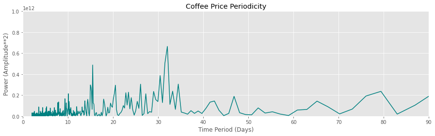

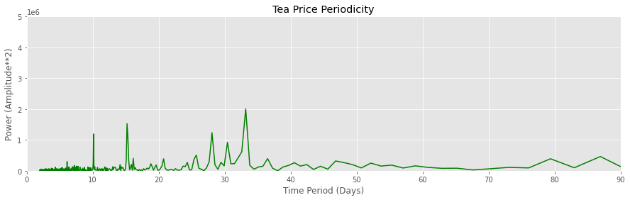
Observations:

The coffee and tea prices have a dominant periodicity of ~ 30 days. This means that the prices rise and fall periodically every 30 days;
咖啡和茶的价格具有约30天的主导周期。这意味着价格每30天定期上涨和下跌；
Smaller peaks are observed at ~15 days and ~ 10 days, which implies that there are also lesser-known periodicities in prices.
在〜15天和〜10天观察到较小的峰值，这意味着价格的周期性也鲜为人知。

警告！ (Warning!)

DFT, and by its extension the FFT, assume that the signal (a.k.a time series) can be composed of a linear sum of sine waves of varying frequencies. This model is actually a linear model and is strictly applicable to stationary signals (those whose statistical properties do not change with time). However, commodity prices in this data are clearly not stationary and seem to be non-linear. So another method must be considered to decompose the time series.

DFT及其扩展FFT假定信号(又名时间序列)可以由频率变化的正弦波的线性和组成。 该模型实际上是线性模型，并且严格适用于平稳信号(其统计属性不会随时间变化的信号)。 但是，该数据中的商品价格显然不是平稳的，而且似乎是非线性的。 因此，必须考虑另一种方法来分解时间序列。

经验模式分解 (Empirical Mode Decomposition)

EMD was first proposed by Norden E. Huang in 1996 as a means to decompose non-linear and non-stationary signals. At the time he was working at NASA as a fluid dynamist.

EMD由Norden E. Huang于1996年首次提出，它是一种分解非线性和非平稳信号的方法。当时他在NASA担任流体力学专家。

EMD is, at its heart, a data-driven adaptive signal decomposition technique. In spirit, it is similar to the Fourier Transform.
EMD本质上是一种数据驱动的 自适应信号分解技术。从本质上讲，它类似于傅立叶变换。
The Fourier Transform tries to break down the signal into a simple linear combination of sine waves of varying frequencies.
傅立叶变换试图将信号分解为频率可变的正弦波的简单线性组合。
The EMD, on the other hand, does not make that assumption, but it needs its intrinsic components to have local frequencies. This makes it extremely useful for dealing with non-linear signals.
另一方面，EMD并未做出该假设，但需要其固有成分具有本地频率。这对于处理非线性信号非常有用。
These intrinsic components are called Intrinsic Mode Functions (IMF) and they represent the various hidden periodicities present in the signal.
这些固有成分称为固有模式函数(IMF) ，它们代表信号中存在的各种隐藏周期。
These IMFs have to satisfy two eligibility criteria — 1) The number of zero-crossing and number of local extrema must differ at most by 1 and 2) the local mean must be close to zero.
这些IMF必须满足两个资格标准-1) 零交叉数和局部极值数最多相差1和2) 局部均值必须接近零。
The process of extracting this IMF from the signal is called sifting and it is done recursively until a suitable stopping criterion is met.
从信号中提取此IMF的过程称为筛选，然后递归进行直到满足合适的停止标准为止。

With the help of sifting and the eligibility criteria, a non-linear and non-stationary signal can be decomposed into its intrinsic components, while maintaining information in the time and frequency domains.

借助于筛选和合格标准，可以将非线性和非平稳信号分解为其固有成分，同时在时域和频域中保持信息。

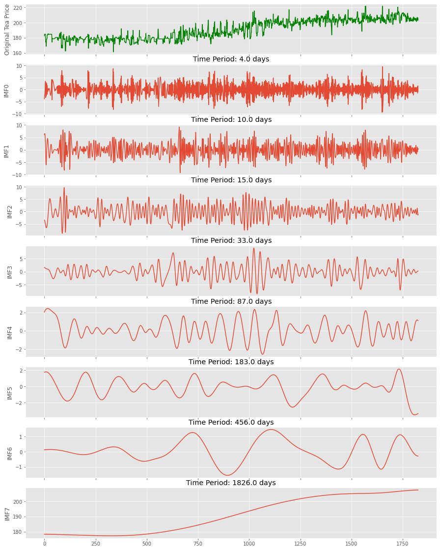
The EMD can be implemented using PyEMD which is the most popular Python library of the lot (and there aren’t many out there for EMD). The FFT algorithm can also be used to extract the dominant frequency in the IMFs generated from the decomposition —

可以使用PyEMD来实现EMD， PyEMD是目前最流行的Python库( 而且EMD并不多 )。 FFT算法还可用于提取由分解产生的IMF中的主频-

emd = EMD()
t = np.arange(0,d0.shape[0]) #Just replace d0: Coffee with d1: Tea
imfs = emd(d0.values, t)fig,ax = plt.subplots(imfs.shape[0]+1, 1, sharex=True, figsize=[15,20])
ax[0].plot(t,d0.values, color='teal')
ax[0].set_ylabel('Original Coffee Price')for i in range(0,imfs.shape[0]):
    ax[i+1].plot(t, imfs[i])
    ax[i+1].set_ylabel('IMF'+str(i))
    sig = imfs[i]
    time_step = 1 #1 Day
    sig_fft = fftpack.fft(sig)
    sample_freq = fftpack.fftfreq(sig.size, d=time_step)
    power = np.abs(sig_fft)
    pos = np.where(sample_freq>0)
    power = power[pos]
    sample_period = 1/sample_freq[pos]
    s = sample_period[np.where(power==power.max())][0]
    ax[i+1].set_title('Time Period: {} days'.format(np.round(s)))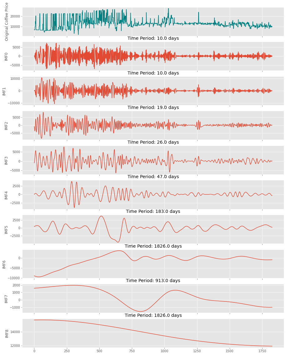

Observations:

The EMD decomposed the coffee price series into several IMFs;
EMD将咖啡价格序列分解为几个IMF。
The last IMF (a.k.a IMF of lowest order) is called the residue and represents the trend;
最后一个IMF( 又称最低顺序的IMF )称为残差，代表趋势。
The residue showed that coffee prices seem to be on a declining trend while the tea prices seem to be increasing;
残留物表明咖啡价格似乎在下降，而茶价格似乎在上升。
Each of the IMF represents hidden periodicity in the prices;
每个基金组织都代表着价格中隐藏的周期性；
The EMD validated the dominant periodicities observed in the initial FFT method and also brought a few additional ones.
EMD验证了在初始FFT方法中观察到的主要周期性，并且还带来了一些其他周期性。

警告！ (WARNING!)

The major concern with the method is that it is difficult to attach physical meaning to the IMFs generated. Since the extraction is data-driven and done recursively from a single signal, there is no well established mathematical framework to make sense of the extracted functions.

该方法的主要问题在于，很难将物理意义附加到生成的IMF上。 由于提取是数据驱动的，并且是从单个信号中递归完成的，因此没有完善的数学框架可以理解提取的函数。

结论 (Conclusion)

Despite its shortcomings, EMD is extremely useful to decompose non-linear and non-stationary signals, without losing information (unlike FFT which is applicable only to linear stationary signals and restricted to the frequency domain)

尽管有缺点，但EMD在分解非线性和非平稳信号而不丢失信息方面非常有用( 与仅适用于线性平稳信号并限于频域的FFT不同 )

I hope this post gave you a flavor of the usefulness of EMD in time series analysis, especially when used in conjunction with FFT.

我希望本文能使您了解EMD在时间序列分析中的有用性，尤其是与FFT结合使用时。