协变量偏移_恶意软件分类的协变量偏移-优快云博客

探讨了数据生成分布中的协变量偏移对模型性能的影响，特别是在恶意软件分类领域。文章分析了输入分布变化对模型泛化能力的挑战，以及如何通过特征工程和先验知识来提高模型对新分布数据的鲁棒性。

摘要生成于 C知道，由 DeepSeek-R1 满血版支持，前往体验 >

协变量偏移

介绍 (Introduction)

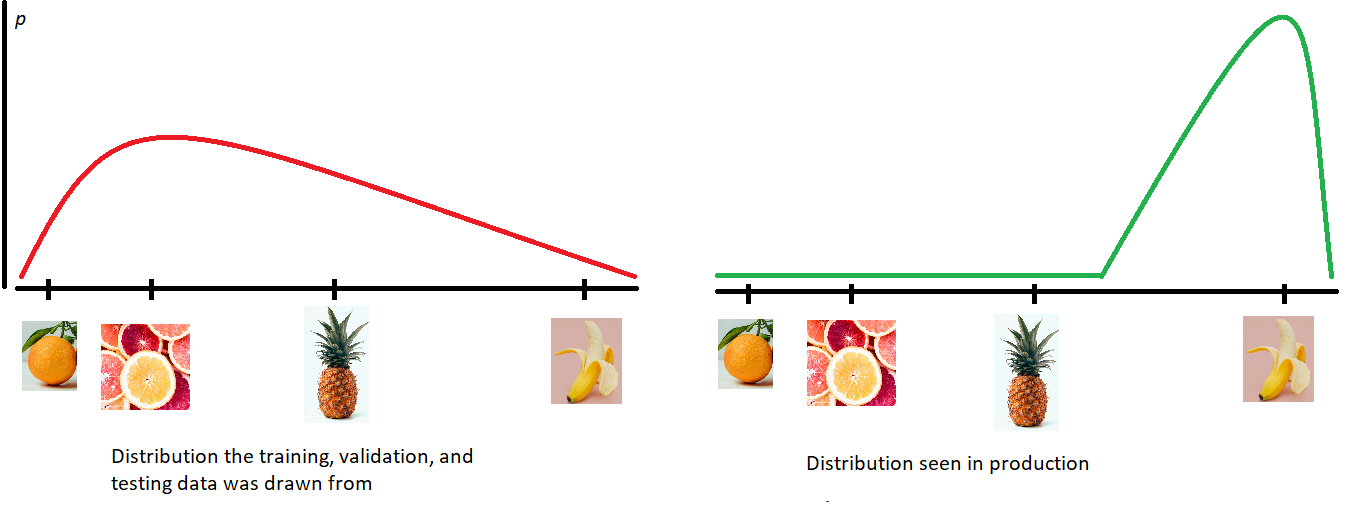
Covariate shift in the data-generating distribution lowers the usefulness of generalization error as a measure of model performance. By unpacking the definitions, the previous sentence translates to “high accuracy on the distribution of files we sampled our training set from (excluding the training set itself) does not always mean high accuracy on other important distributions (even if the true relationship between a sample and its label does not change).” A fruit classifier that had a single example of a banana in its training set might perform poorly on a sample set consisting solely of 10,000 variations of bananas, even if it did very well on a held-out test set sampled from the same distribution as its training set (where presumably bananas are scarce). This performance gap can be a problem because approximating generalization error with a held-out test set is the canonical way to measure a model’s performance.

数据生成分布中的协变量偏移降低了泛化误差作为模型性能度量的有用性。通过解压缩定义，前一句翻译为“从中抽取训练集的文件分布的准确性很高(不包括训练集本身)，并不总是意味着其他重要分布的准确性很高(即使样本之间的真实关系也是如此)并且其标签不变。” 在训练集中仅包含一个香蕉示例的水果分类器，在仅包含10,000个香蕉变体的样本集上，即使在与该样本相同分布的抽样测试集上做得非常好，其效果也可能很差训练集(大概缺少香蕉)。这个性能差距可能是一个问题，因为使用保留的测试集来近似泛化误差是衡量模型性能的规范方法。

Image for post — A rapidly changing input distribution is a common challenge in practical machine learning

This concept is essential for malware classification, and many papers discuss it in the context of sampling bias, where the samples used for training are not randomly sampled from the same distribution as the samples used for testing. Anecdotally, the intuition that models with good generalization may have poor performance once deployed — due to the difference between the files the model was trained on and the files it scans — is held by many malware analysts I’ve worked with, including those with little ML experience. However, it’s not always clear how to identify and fix issues related to covariate shift: conventional regularization techniques that improve generalization may not help when good generalization isn’t enough. After spending 5 years reverse engineering and classifying malware (using traditional, non-ML based techniques), I developed lots of intuitions about malware classification that I wasn’t able to express until I grew a passion for machine learning. My goal with this blog is to explain these opinions in the more formal context of machine learning. As some of these attempts at formal explanations are imprecise (and possibly incorrect), another goal of this blog is to solicit discussion, feedback, and corrections. I pack in a lot of different concepts and background because I feel relating concepts to each other helps improve understanding, especially if they can be tied back to practical goals like malware classification.

这个概念对于恶意软件的分类至关重要，许多论文在抽样偏差的背景下进行了讨论，在抽样偏差中，用于训练的样本不是从与用于测试的样本相同的分布中随机抽样的。有趣的是，由于模型的训练文件和扫描的文件之间存在差异，具有良好普遍性的模型一旦部署可能会导致性能下降，直觉是由我工作过的许多恶意软件分析师(包括那些分析很少的人)持有的。 ML经验。但是，并不总是很清楚如何识别和修复与协变量移位相关的问题：如果良好的概括性不够，传统的提高泛化性的正则化技术可能无济于事。经过5年的逆向工程和对恶意软件分类(使用传统的非基于ML的技术)后，我开发了许多关于恶意软件分类的直觉，直到对机器学习充满热情之前，我一直无法表达这些直觉。我在此博客中的目标是在更正式的机器学习环境中解释这些观点。由于其中一些尝试进行正式解释的方法不准确(并且可能不正确)，因此本博客的另一个目标是征求讨论，反馈和更正。我打包了许多不同的概念和背景，因为我觉得将概念相互关联有助于增进理解，尤其是如果可以将它们与诸如恶意软件分类之类的实际目标联系起来的话。

I hope that anyone interested in covariate shift can benefit from this blog, but the target audience is a person with some experience in machine learning who wants to apply it to computer security-related tasks, particularly “static” malware classification (where we want to classify a file given its bytes on disk, without running it). One of the key conclusions that I hope this blog supports is the importance of incorporating prior knowledge into a malware classification model. I believe prior knowledge is particularly relevant when discussing the ways a model might represent its input before the classification step. For example, I detail some domain knowledge that I believe is relevant to CNN malware classification models in this article: https://towardsdatascience.com/malware-analysis-with-visual-pattern-recognition-5a4d087c9d26#35f7-d78fef5d7d34

我希望对协变量转换感兴趣的任何人都可以从此博客中受益，但是目标受众是具有一定机器学习经验的人，他希望将其应用于与计算机安全相关的任务，尤其是“静态”恶意软件分类(在此我们希望根据文件在磁盘上的字节数对文件进行分类，而不运行它)。我希望该博客支持的主要结论之一是将先验知识整合到恶意软件分类模型中的重要性。我认为在讨论模型在分类步骤之前可能表示其输入的方式时，先验知识尤其重要。例如，在本文中，我详细介绍了一些我认为与CNN恶意软件分类模型有关的领域知识： https : //towardsdatascience.com/malware-analysis-with-visual-pattern-recognition-5a4d087c9d26#35f7-d78fef5d7d34

I’ve included an appendix that provides additional background by going over some core concepts used in the main section (such as inductive bias, generalization, and covariate shift)

我提供了一个附录，该附录通过介绍主要部分中使用的一些核心概念(例如归纳偏差，泛化和协变量平移)提供了其他背景。

恶意软件分类的协变量偏移 (Covariate Shift in Malware Classification)

I do not think models that demonstrate good generalization on large sample sets are useless. If a model does not perform well on the distribution it was trained on, that’s a problem. There is plenty of empirical evidence in the security industry that a model that generalizes well without being super robust to changes in the input distribution can still provide value, especially if retrained frequently and targeted at specific customer environments. However, at this point, many models used in the industry demonstrate high accuracy on held-out test sets. I believe improving performance on samples from important new distributions, such as files created a month after the model was trained, has a more practical impact than making tiny marginal improvements in test set accuracy. The next few sections go over why these new distributions are essential and why they are an example of “covariate shift.” If you’re new to the concept of covariate shift, I’d recommend going through the background section in the appendix.

我认为对大型样本集进行良好概括的模型并不是没有用的。如果模型在经过训练的分布上表现不佳，那就是一个问题。在安全行业中，有大量的经验证据表明，一种模型能够很好地泛化而不会对输入分布的变化具有超强的鲁棒性，但仍然可以提供价值，尤其是在经常进行重新培训并针对特定客户环境的情况下。但是，在这一点上，行业中使用的许多模型在保留的测试集上都显示出很高的准确性。我相信，提高重要的新发行版中样本的性能(例如在训练模型后一个月创建的文件)，比对测试集准确性进行微不足道的改善具有更大的实际影响。接下来的几节将介绍为什么这些新分布是必不可少的，以及为什么它们是“协变量转变”的一个示例。如果您不熟悉协变量移位的概念，我建议您仔细阅读附录中的背景部分。

为什么p(x)变化 (Why p(x) changes)

In the case of malware classification, p(x) is the distribution of binary files analyzed by the model. Practical malware classifiers are never applied to the distribution they are trained on; they need to perform well on sets of samples in production environments that are continually evolving. For many antivirus vendors, that means performing well on files present on every machine with that antivirus, as well as samples submitted to other services like VirusTotal and antivirus review tests. There are two main reasons why generalization performance may not be a good predictor of how well a model performs on these samples:

对于恶意软件分类， p(x)是模型分析的二进制文件的分布。实用的恶意软件分类器永远不会应用于对其进行训练的发行版；他们需要在不断发展的生产环境中对一组样本执行良好的操作。对于许多防病毒供应商而言，这意味着在具有该防病毒功能的每台计算机上存在的文件以及提交给其他服务(如VirusTotal和防病毒查看测试)的示例上，都表现出色。泛化性能可能不能很好地预测模型在这些样本上的表现，主要有两个原因：

Sample selection bias: It is rare in the security industry to train models on a random selection of files that the model encounters when deployed. This is because accurate labeling is expensive: it often requires some level of manual human analysis, and it requires having access to all scanned files. It is normal to include files that analysts have labeled for other reasons, such as for the direct benefit of customers or files that have been supplied and labeled by third parties. If human analysis isn’t involved, there is a danger of feedback loops between multiple automated analysis systems. Because we can’t feasibly train the model on a truly random sample of the target distribution, the sample selection process is biased. Technically we can get around this by randomly sampling files our scanner encounters and labeling them with human analysts, but this would result in a small sample set of mostly clean files. I refer to the distribution of files that are encountered by the scanner after the model has been deployed as the “in-production distribution.”

样本选择偏差：在安全行业中，很少会在部署模型时随机选择模型时训练模型。这是因为准确的标签非常昂贵：通常需要进行一定程度的手动人工分析，并且需要访问所有扫描的文件。通常包含分析人员出于其他原因而标记的文件，例如为了客户的直接利益或由第三方提供并标记的文件。如果不进行人工分析，则存在多个自动化分析系统之间存在反馈循环的危险。因为我们无法在目标分布的真正随机样本上训练模型，所以样本选择过程存在偏差。从技术上讲，我们可以通过对扫描仪遇到的文件进行随机采样并使用人工分析人员对其进行标记来解决此问题，但这将导致生成一小部分样本，其中大部分为干净文件。我将模型部署后，扫描程序遇到的文件分发称为“生产中分发”。

Environment shift: Every time you copy, edit, update, download, or delete a file, you modify the distribution your malware scanner encounters. When summed across every machine, the shift in distribution can be significant enough to mean a classifier that performed well last week may degrade significantly this week. Malware classifiers also exist in an adversarial setting, where attackers make deliberate modifications to the input to avoid the positive classification. A typical strategy to mitigate this issue is constant retraining, but it is impossible to ever train on the actual in-production distribution (even if we did have labels for them) unless we never scan files created after we gathered our training set. This scenario produces a type of sample selection bias that is impractical to overcome: we cannot train on samples that will be created in the future.

环境转变：每次复制，编辑，更新，下载或删除文件时，您都会修改恶意软件扫描程序遇到的分布。如果将每台机器的总和相加，分布的变化可能会非常明显，这意味着上周表现良好的分类器可能会在本周大幅下降。恶意软件分类器也存在于对抗环境中，攻击者在其中故意对输入内容进行修改，以避免正面分类。缓解此问题的一种典型策略是不断地进行再培训，但是除非在收集培训集之后再也不扫描创建的文件，否则就不可能对实际的生产发行版进行培训(即使我们确实有标签)。这种情况会产生一种无法克服的样本选择偏见：我们无法训练将来将要创建的样本。

为什么p(y | x)不变 (Why p(y|x) does not change)

Covariate shift requires that p(y=malicious|x=file) does not change when p(x) does (see appendix). In the case of malware classification, p(y = malicious|x) is the probability a given file x is malicious. If p(y|x) and p(x) both change, it may be impossible to maintain accuracy. I can’t prove p(y|x) won’t change, but I argue that changes are generally, for certain classes of models, independent of p(x). Here p refers to the true data-generating distributions rather than a probabilistic classifier’s attempt to approximate p(y|x).

There are two main reasons why p(y=malicious|x) would be anything other than 1 or 0:

p(y = malicious | x)不是1或0的原因有两个主要原因：

A. Uncertainty in the input: y is a deterministic function of some representation x’, but the input x the model uses does not contain all the relevant parts of x’. This concept is touched upon in the “deterministic vs stochastic classification” section in the appendix, but it’s a critical case, so I’ll expand on it in the next section. I use x’ to refer to inputs that can be mapped deterministically to a label and x to refer inputs that may or may not be deterministically mappable to a label.

A.输入中的不确定性： y是某些表示x'的确定性函数，但是模型使用的输入x并不包含x'的所有相关部分。附录的“确定性与随机分类”一节中涉及了此概念，但这是一个关键案例，因此我将在下一节中对其进行扩展。我用x”至指可以确定性地被映射到一个标签，并且x是指输入，其可以是或可以不是可映射确定性到标签输入。

B. Uncertainty in the label: The definition of y does not fully account for all inputs (grayware is an example in malware classification). I’ll leave a full explanation to the appendix section “Why p(y|x) does not change: Uncertainty in the label.”

B.标签中的不确定性： y的定义并未完全考虑所有输入(灰色软件是恶意软件分类中的一个示例)。我将对附录部分“为什么p(y | x)不变：标签中的不确定性”进行完整的解释。

输入的不确定性 (Uncertainty in the input)

In this part, I argue that the bytes in a file correspond to x’.

在这一部分中，我认为文件中的字节对应于x'。

Here’s a simple example. I precisely define ‘eight’ to be a specific shape shown in Figure 1

这是一个简单的例子。我将“八”精确定义为如图1所示的特定形状

Figure 1: The definition of ‘eight’

图1：“八”的定义

and ‘three’ to be the shape shown in Figure 2

和“三个”的形状如图2所示

Figure 2: The definition of ‘three’

图2：“三个”的定义

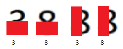
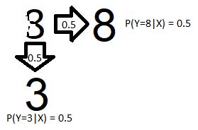
If we have access to the entire input (x’ = Figure 1 or Figure 2), we know with perfect certainty what the label should be. However, we may not have access to the full input as illustrated below, where some of the input is hidden with a red box:

如果我们可以访问整个输入( x' =图1或图2)，则可以完全确定地知道标签应该是什么。但是，我们可能无法访问完整的输入，如下所示，其中某些输入用红色框隐藏：

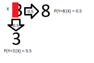
In this case, our input x (Figure 3) maps stochastically (Figure 4) to two different x’ (Figure 1,2), which map deterministically to the y values ‘eight’ and ‘three’. I’ll refer to the mapping function as g, in this case, g adds a red box that hides the difference between an eight and three. I refer to the function that maps x’ to y as f_true, which is effectively a perfect classifier that avoids randomness by having access to all relevant information. See the ‘deterministic vs stochastic classification’ section in the appendix for more details.

在这种情况下，我们的输入x (图3)随机映射(图4)到两个不同的x' (图1,2)，它确定性地映射到y值“八”和“三”。我将映射函数称为g ，在这种情况下， g添加了一个红色框，该框隐藏了8与3之间的差异。我将将x'映射到y的函数称为f_true ，这实际上是一个完美的分类器，可以通过访问所有相关信息来避免随机性。有关更多详细信息，请参见附录中的“确定性分类与随机分类”部分。

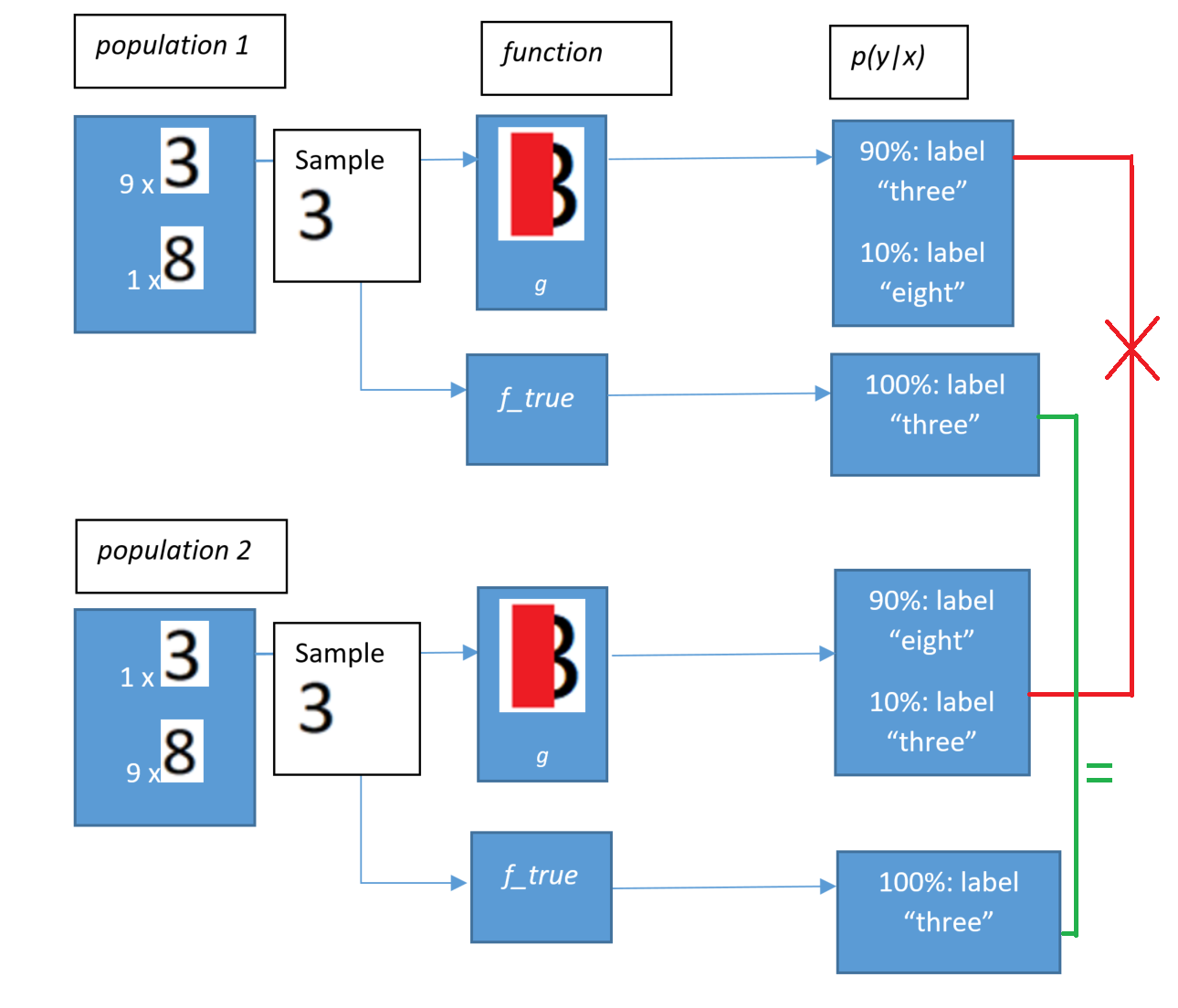
If the training set contains 90 copies of Figure 3 labeled as “3” and 10 copies labeled as “8” and we have a uniform prior, then p(y=8|Figure 3) = 0.1 and p(y=3|Figure 3) = 0.9. If the test set is sampled from the same distribution, it is likely to have a similar ratio of 3’s to 8’s, so our model will generalize well. However, a new-distribution test set might have 8’s appear 9 times as much as 3’s on average. If we tested on a sample from that distribution, we would probably get abysmal performance. Unless we can un-hide some of the data, it may not be feasible to have good generalization error and new-distribution error. In this blog, I use new-distribution error to refer to the equivalent of generalization error when the model is applied to a distribution different than the one its training set was sampled from (more on this in the covariate shift section of the appendix). Practically, attempting to find the new-distribution error for the in-production distribution is likely a better measure of performance for a malware classifier than the generalization error. Figure 5 illustrates this example. A key takeaway is that when we transition from population 1 to population 2, we undergo covariate shift when considering our raw sample (figure 2 in both cases) and p(y|x) defined by f_true. However, the type of shift we encounter when we consider an intermediate representation that hides relevant information (figure 3) isn’t covariate shift: it’s worse than covariate shift. This is because p(y=label “three”|x=figure 3) goes from 90% in population 1 to 10% in population 2.

如果训练集包含90个标记为“ 3”的图3副本和10个标记为“ 8”的副本，并且我们具有统一的先验，则p(y = 8 |图3)= 0.1和p(y = 3 |图) 3)= 0.9 。如果测试集是从相同的分布中采样的，则它的3与8的比率可能相似，因此我们的模型可以很好地推广。但是，新发行的测试集可能出现8的概率是平均3的9倍。如果我们对该分布的样本进行测试，则可能会获得糟糕的性能。除非我们能取消隐藏某些数据，否则具有良好的泛化误差和新分布误差可能是不可行的。在本博客中，当模型应用于不同于其训练集样本的分布时，我使用new-distribution错误来指代泛化错误(有关更多信息，请参见附录的协变量平移部分)。实际上，与泛化错误相比，尝试找到生产中分发的新分发错误可能是衡量恶意软件分类器性能的更好指标。图5说明了此示例。一个关键的要点是，当我们从总体1过渡到总体2时，在考虑原始样本(两种情况下均为图2)和f_true定义的p(y | x)时，我们会发生协变量偏移。但是，当我们考虑隐藏相关信息的中间表示形式时，我们遇到的变化类型(图3)不是协变量变化：它比协变量变化差。这是因为p(y =标签“三” | x =图3)从人口1的90％变为人口2的10％。

In summary: If information is hidden (input is g(x’)) then p(y|x) may change with p(x) because the change to p(x) is caused by the underlying distribution p(x’) changing. This change in p(y|x) can occur when there’s sampling bias or environment shift, which are both common in malware classification.

总结：如果信息是隐藏的(输入为g(X '))，那么P(Y | X)可以与P(X)，因为变化至p(x)由下面的分布p(X引起的改变')改变。 p(y | x)的这种变化可能在存在恶意软件分类中常见的采样偏差或环境偏移时发生。

As an example, say your dataset consisted of many recent malicious samples, along with clean samples from a wide range of dates. Given that malicious samples change more frequently than clean samples, this is a common situation. Say the model uses the (PE) file’s timestamp value to classify the files (g hides all information except the timestamp). This feature works equally well for the training set and test sets sampled from the same distribution, as in both cases, malware tends to be more recent than clean files. The feature technically generalizes well, but any classifier that is based entirely on timestamp will not perform well when a dataset contains recent clean files, such as on any machine that just had a software update. To relate this to the deterministic vs stochastic classification section of the appendix, y=f_ideal(x = PE Timestamp) is very different from y=f_true(x’ = all bytes in a file), where x = g(x’) and g is a feature extractor that extracts the PE file’s timestamp. Note this assumes the malicious samples do not make deliberate modifications to the PE timestamp, which can happen.

举例来说，假设您的数据集包含许多近期的恶意样本以及日期范围广泛的干净样本。鉴于恶意样本比干净样本更频繁地发生更改，这是一种常见情况。假设模型使用( PE )文件的时间戳值对文件进行分类( g隐藏除时间戳之外的所有信息)。此功能对于从同一分发中采样的训练集和测试集同样有效，因为在两种情况下，恶意软件往往比干净文件更新。从技术上讲，该功能的泛化效果很好，但是当数据集包含最新的干净文件时，例如在刚刚进行了软件更新的任何计算机上，任何完全基于时间戳的分类器都无法正常运行。要将其与附录的确定性分类与随机分类部分相关， y = f_ideal(x = PE Timestamp)与y = f_true(x'=文件中的所有字节 )有很大不同，其中x = g(x')和g是一个功能提取器，用于提取PE文件的时间戳。请注意，这是假设恶意样本未对PE时间戳进行故意修改，而这可能会发生。

保持p(y | x)恒定所需的假设 (Required assumption to keep p(y|x) constant)

The definition of malware is precise, unchanging, and is dependent solely on the bytes of a file (x’), so that y is a deterministic function of x: p(y = malicious|x’) = 1 or 0 = f_true(x’ = all bytes in a file). Here’s another way to think about that: given that the space of files that can be practically represented is finite (though absurdly large), we can give a label to every point in that space. This assumption requires that we consider a file in the context of its dependencies, as some types of malware have multiple components.

恶意软件的定义是精确的，不变的，并且仅取决于文件( x' )的字节，因此y是x的确定性函数： p(y =恶意| x')= 1或0 = f_true( x'=文件中的所有字节)。 这是另一种思考方式：鉴于实际上可以表示的文件空间是有限的(尽管非常大)，所以我们可以为该空间中的每个点都加上标签。这种假设要求我们在文件依赖关系的范围内考虑文件，因为某些类型的恶意软件具有多个组件。

In the next part, I discuss ways to try and determine if an approach is more or less vulnerable to changes in input distribution. There is always some vulnerability, as our classifiers need dimensionality reduction, and we don’t have dimensionality reduction techniques that won’t lose at least some information relevant to the deterministic mapping from x’ to y (f_true).

在下一部分中，我将讨论尝试确定一种方法是否或多或少容易受到输入分布变化的影响的方法。总会有一些漏洞，因为我们的分类器需要降维，而我们没有降维技术，这些技术不会丢失至少一些与从x'到y(f_true)的确定性映射有关的信息。

缓解因协变量移位引起的问题 (Mitigating Issues Caused By Covariate Shift)

After making some assumptions, the previous section established that covariate shift is an ok way to describe what happens when we consider all the bytes in a file and the distribution of files changes. Unlike scenarios where both p(x) and p(y|x) change, we have a path to creating a classifier that works: find a function as close as possible to f_true. Here’s another way to look at that: probabilistic classifiers attempt to find p(y=label|x’=bytes in a file). The data generating distribution has a p(y|x’) = f_true which does not change when p(x’) changes. If we find f_true, then our model’s p(y|x’) will not change with changes in p(x’).

在做出一些假设之后，上一节确定了协变量移位是描述当我们考虑文件中的所有字节并且文件的分布发生变化时发生的情况的一种好方法。与p(x)和p(y | x)都改变的情况不同，我们有一条创建有效的分类器的途径：找到一个尽可能接近f_true的函数 。这是另一种看待方式：概率分类器尝试查找p(y = label | x'=文件中的字节)。 数据生成分布具有p(y | x')= f_true ，当p (x')更改时，该值不变。如果找到f_true，则模型的p(y | x' )将不会随着p(x')的变化而改变。

An alternative might be trying to predict precisely where the input distribution will shift, but I’m skeptical of how well that would work in a highly dynamic, adversarial setting. In the fruit classifier example from the introduction, trying to model f_true would mean creating a model that understood the definition of each fruit and was able to compare any input to that definition: this approach would work when the dataset shifts to mostly bananas. Predicting where the input distribution will shift might means putting a higher emphasis on a specific class during training. If we picked a class other than bananas, our model would still perform poorly after the input distribution shifts to mostly bananas.

一种替代方法可能是尝试精确地预测输入分布将在何处变化，但我对在高度动态的对抗环境中这种方法的效果持怀疑态度。在引言的水果分类器示例中，尝试对f_true进行建模将意味着创建一个模型，该模型可以理解每个水果的定义，并且能够将任何输入与该定义进行比较：当数据集转移到大多数香蕉时，此方法将起作用。预测输入分布将向何处转移可能意味着在培训期间将重点放在特定的班级上。如果我们选择香蕉以外的其他类别，则在输入分布转移到大部分为香蕉之后，我们的模型仍然会表现不佳。

是什么使模型容易受到协变量偏移的影响，又该如何解决？ (What makes a model vulnerable to covariate shift, and how can that be fixed?)

Hypothetically a new-distribution dataset sampled randomly from the files scanned by a deployed model could be used to measure relevant new-distribution error. Receiving more false-positive reports than expected given the test set error may also hint at high new-distribution error. However, as perfect generalization does not guarantee robustness to changes in the input distribution (see the PE timestamp example in the previous part), the strategies that can be used to increase generalization such as common regularization techniques will not help past a certain point (though if our model doesn’t generalize that’s bad news for new-distribution performance). We need to find a new knob to turn to improve the new-distribution error once we have a low generalization error. I think that one of the best ways to do that is to find ways to incorporate prior knowledge to get the best inductive bias. There are several ways to restrict the hypothesis space of our learner to exclude models that generalize well but perform poorly on the new-distribution test set. In the example where the timestamp is used as a feature to produce a model that generalizes but is not robust to changes in the input distribution, excluding hypotheses that rely on the PE timestamp may help reduce new-distribution error. This exclusion is based on the prior knowledge that clean and malicious files can both be new or old. For PE files, there are a huge number of features that may need to get excluded, and features we want to keep may be difficult to compute (though it may be possible to use neural networks as feature extractors for more complicated functions).

假设从部署模型扫描的文件中随机采样的新分布数据集可用于测量相关的新分布错误。在给定测试集错误的情况下，收到比预期更多的假阳性报告也可能暗示着较高的新分布错误。但是，由于完美的泛化并不能保证输入分布变化的鲁棒性(请参阅上一部分的PE时间戳示例)，因此可以用于增强泛化的策略(例如常规正则化技术)将无济于事(尽管如果我们的模型不能一概而论，那对于新发行版的效果来说是个坏消息)。一旦泛化误差很低，我们需要找到一个新的旋钮来改善新分布误差。我认为做到这一点的最佳方法之一就是找到方法，以结合先验知识以获得最佳归纳偏差。有几种方法可以限制我们的学习者的假设空间，以排除在新分布测试集上泛化能力强但表现不佳的模型。在以时间戳为特征的示例中，该模型可以推广但对输入分布的变化不具有鲁棒性的模型，排除依赖于PE时间戳的假设可能有助于减少新分布误差。此排除基于现有知识，即干净和恶意文件可能是新文件也可能是旧文件。对于PE文件，可能需要排除大量特征，而我们想要保留的特征可能难以计算(尽管可能将神经网络用作更复杂功能的特征提取器)。

In the extreme, if we have prior knowledge of the function y = f_true(x’) that maps x’ to y across the entire domain of x’, then we can exclude all hypotheses that are not f_true(x’). While this function is generally not practical to find, it is required for malware analysts to be able to mentally approximate f_true to be able to classify all files they see, even if they haven’t seen similar files before. It helps that in practice, we don’t need to consider the whole domain of possible files, just all files created by modern humans and our tools.

在极端情况下，如果我们有函数y = f_true(X“)的事先知道地图X”跨x的整个域Y“那么我们就可以排除不f_true(X所有假设”)。 尽管通常很难找到此功能，但恶意软件分析人员必须能够从心理上近似f_true才能对他们看到的所有文件进行分类，即使他们之前从未见过类似文件。它在实践中有帮助，我们不需要考虑可能文件的整个领域，只需考虑由现代人及其工具创建的所有文件。

We can (and probably should) incorporate inductive bias at every step: what data to use, how to preprocess it, what model to use, how to pick architecture, features, hyperparameters, training method, etc. An example of each of these is beyond the scope of this blog; instead, I’m going to focus on feature extraction, which is one of the most popular ways to introduce inductive bias.

我们可以(可能应该)在每个步骤中合并归纳偏差：使用哪些数据，如何对其进行预处理，使用哪种模型，如何选择体系结构，功能，超参数，训练方法等。每个示例都是超出本博客的范围；相反，我将专注于特征提取，这是引入归纳偏差的最流行方法之一。

实现输入分布变化的鲁棒性 (Achieving robustness to changes in the input distribution)

Feature engineering is a crucial step for many types of models as features contribute directly to the inductive bias of the model: if features exclude parts of the input data, the model cannot use that data as part of the learned hypothesis. Transforming the data into a lower-dimensional set of features is also very important, as one of the main challenges in finding f_true(x’) is that x’ is very high dimensional: a major problem for many types of classifiers. Hand engineered features are common for some models like random forests, while other models like convolutional neural networks automatically extract features. For both hand-engineered and automatically extracted features, models tend to follow the architecture shown in Figure 6:

对于许多类型的模型而言，特征工程是至关重要的一步，因为特征直接导致模型的归纳偏差：如果特征排除了输入数据的一部分，则模型无法将该数据用作学习的假设的一部分。将数据转换为低维特征集也非常重要，因为找到f_true(x')的主要挑战之一是x'的维数很高：这是许多类型分类器的主要问题。手工设计的特征在某些模型(例如随机森林)中很常见，而在其他模型(例如卷积神经网络)中会自动提取特征。对于手工设计的特征和自动提取的特征，模型倾向于遵循图6所示的体系结构：

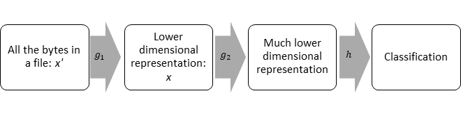
Each box depends entirely on the previous box. The first three boxes contain groups of features or a ‘representation.’ Boxes toward the right cannot contain more information about the input than boxes to their left. Typically, the goal of an architecture like this is to throw away information that is irrelevant to the classification. Less irrelevant information allows the classifier to deal with a lower-dimensional representation than x’ while maintaining performance. Specifics depend on the model, with neural networks having many more layers of representation than decision tree-based models, for example. The critical detail is that each representation tends to have less information about the input than the previous representation, and if the information lost is relevant to f_true(x’), then all downstream portions of the model have to deal with the ‘Uncertain input’ case, where I argued that p(y|x) could change with p(x). Therefore, we want to ensure the lower-dimensional representation still contains enough information to compute f_true(x’) (see Figure 7), even though it contains less information about the original input overall. Unfortunately, we usually can’t achieve this in practice, so when considering a model’s intermediate representation of the input, we’re no longer dealing with covariate shift. That said, we can still work to mitigate the amount p(y|x=intermediate representation) changes with p(x).

每个框完全取决于前一个框。前三个框包含要素组或“制图表达”。与左侧的框相比，右侧的框不能包含有关输入的更多信息。通常，这样的体系结构的目标是丢弃与分类无关的信息。较少的不相关信息使分类器可以处理比x'低的维表示，同时保持性能。具体细节取决于模型，例如，神经网络具有比基于决策树的模型更多的表示层。关键的细节是，每个表示形式都比以前的表示形式具有更少的输入信息，如果丢失的信息与f_true(x')有关 ，则模型的所有下游部分都必须处理“不确定的输入”情况下，我认为p(y | x)可能随p(x)改变。因此，我们希望确保低维表示形式仍然包含足够的信息来计算f_true(x')(请参见图7)，即使它包含的总体原始输入信息较少。不幸的是，在实践中我们通常无法实现这一点，因此，当考虑模型的输入中间表示时，我们将不再处理协变量偏移。这就是说，我们仍然可以工作，以减轻的量P(Y | X =中间表示)与P(X)变化。

As discussed in the paper “Why does deep and cheap learning work well”, this concept is related to the data processing inequality:

正如论文“为什么深度学习和廉价学习很好地起作用”中所讨论的，该概念与数据处理不平等有关：

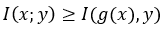
>= is replaced by = if g(x) is a sufficient statistic for y. Mutual information (I) is distribution-specific, so even if g(x) is a sufficient statistic for y given p(x), it may not be when the distribution shifts to p’(x). To be perfectly robust to change in the input distribution, we need y to be a deterministic function of g(x). If that’s the case, g(x) is a sufficient statistic for y for all distributions over x. We already established that this is the case for the data-generating distribution: covariate shift implies that p(y|x’) does not change with p(x’).

如果g(x)对于y是足够的统计量，则将> =替换为= 。互信息( I)是特定于分布的，因此即使g(x)对于给定p(x)的 y来说是足够的统计量，当分布转移到p'(x)时也可能不是。为了完全鲁棒地改变输入分布，我们需要y是g(x)的确定性函数。如果真是这样，对于x上的所有分布， g(x)都是y的足够统计量。我们已经确定数据生成分布就是这种情况：协变量移位意味着p(y | x')不会随p(x')改变。

Classification is discussed in ‘deep and cheap learning’ paper as the reverse of a Markov chain-based generation procedure, which makes intuitive sense for malware classification: the author(s) of a file will know if the functionality they programmed is malicious or not as an early step in the creation process. An example of reversing the process for malware is shown in Figure 8:

分类在“深入而廉价的学习”文章中进行了讨论，与基于马尔可夫链的生成过程相反，这对于恶意软件分类具有直观的意义：文件的作者将知道他们编写的功能是否为恶意软件作为创建过程的第一步。逆转恶意软件过程的示例如图8所示：

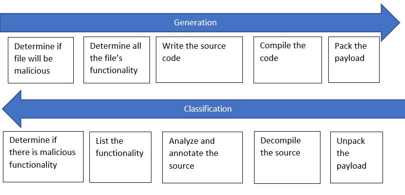
There are shortcuts analysts use to speed up classification, but this diagram is not too far off from the engineering and reverse engineering that goes into malware creation and human analysis (if the analyst wants the most accurate result and has a lot of time). Unfortunately, each of these steps is complicated, and creating a robust function to transition between them is probably impractical today — malware packers are still the default way to hide from antivirus products. We need an alternative, but it helps to keep this roughly idealized Markov chain in mind: note that at no step in the classification process is information relevant to malicious functionality lost. In a later blog, I may discuss alternatives inspired by the shortcuts malware analysts use to speed up classification, with a focus on malware packers.

分析人员可以使用一些快捷方式来加快分类速度，但是该图与恶意软件创建和人工分析所涉及的工程和逆向工程相差不远(如果分析人员希望获得最准确的结果并且有很多时间)。不幸的是，每个步骤都很复杂，并且创建强大的功能以在它们之间进行转换在当今可能不切实际-恶意软件打包程序仍然是对防病毒产品隐藏的默认方法。我们需要一种替代方法，但它有助于牢记这种大致理想化的马尔可夫链：请注意，分类过程中的任何步骤都不会丢失与恶意功能相关的信息。在以后的博客中，我可能会讨论受恶意软件分析人员用来加快分类速度的快捷方式启发的替代方法，重点是恶意软件打包程序。

The key takeaway is that if a representation the model uses at any point does not contain information directly related to the file being malicious or not, the model may be more vulnerable to changes in the input distribution. For example, some models in the security industry primarily use values extracted from the PE header as features. However, this representation excludes a lot of information related to f_true(x’), as prior knowledge tells us PE header values do not give much indication about a file’s behavior, which is required to determine if the file is malicious. This is compounded by the fact that the default way to evade antivirus signatures — custom malware packers — can set the PE header to pretty much whatever they want. A model that depends entirely on PE header values may do a good job detecting files packed with malware packers present in its training set, but will likely do worse when presented with a new malware packer. A representation that includes a file’s possible behaviors, however, would not throw away information related to f_true(x’). This is difficult to do in the context of static detection (detection without executing the file); however, we can still use prior knowledge to try and extract features that are more closely related to f_true(x’) than PE header data. An example of this is a feature that detects obfuscated data, as obfuscation is often applied to make antivirus detection more difficult: something only malware needs to do.

关键要点在于，如果模型在任何时候使用的表示形式都不包含与是否存在恶意文件直接相关的信息，则模型可能更容易受到输入分布更改的影响。例如，安全行业中的某些模型主要使用从PE标头中提取的值作为特征。但是，此表示法排除了许多与f_true(x')相关的信息，因为先验知识告诉我们PE标头值并未提供太多有关文件行为的指示，而这是确定文件是否为恶意文件所必需的。逃避防病毒签名的默认方法(自定义恶意软件打包程序)可以将PE标头设置为几乎任何所需的值，这使情况更加复杂。完全依赖于PE标头值的模型可以很好地检测其训练集中存在恶意软件打包器的文件，但是当出现新的恶意软件打包器时，其性能可能会更差。但是，包含文件可能行为的表示形式不会丢弃与f_true(x')相关的信息。在静态检测(不执行文件的检测)的情况下很难做到这一点；但是，我们仍然可以使用先验知识来尝试提取与PE标头数据相比与f_true(x')更紧密相关的特征。这样的一个示例是检测混淆数据的功能，因为混淆通常被用来使反病毒检测更加困难：只有恶意软件才需要做。

The problem of throwing away information relevant to the data-generating distribution’s p(y|x’) was also illustrated back in figure 5: by hiding important data with a function g, a model that’s built on top of g’s representation will often have the relation between g(x’) and the label change when the raw input distribution p(x’) changes.

丢弃与数据生成分布的p(y | x')相关的信息的问题在图5中也得到了说明：通过使用函数g隐藏重要数据，建立在g表示之上的模型通常具有当原始输入分布p(x')改变时， g(x')与标签之间的关系也会改变。

结论/未来工作 (Conclusion/Future Work)

Given that there are a lot of tools focused on improving generalization, it may be helpful to think about how we can tie generalization error to improving robustness to changes in the input distribution. If our samples are represented in a way that makes malicious files from a new distribution appear the same as malicious files from our original distribution, lowering generalization error may be all that’s necessary. I plan to discuss some ways to approach robustness to changes in input distribution in another blog, with a focus on representation. One example is using convolutional neural networks to specifically detect visual features in a file that human analysts would immediately recognize as malicious across any distribution of files, but for which it would be difficult to manually program heuristics. I would also like to find good methods for measuring new-distribution error for better model comparison. Some distributions are clearly better than others for measuring new-distribution error, and the practical problem of finding the true label of all in-production samples still prevents that distribution from being used in practice. For example, an alternative could be finding the true labels for a small subset (<1000) of samples from the in-production distribution and calculating accuracy (or precision) along with a confidence interval that accounts for the limited sample set. Precision is often easier to work within the security industry due to difficulty in finding in-production false negatives in an unbiased way (due to the number of true negatives), and the fact that false positives on average negatively impact more people than false negatives (clean files are much more likely to appear on more than one machine). I would also like to consider adversarial machine learning in the context of covariate shift.

鉴于有许多工具专注于改善泛化，因此思考如何将泛化误差与输入分布变化的鲁棒性联系起来可能会有所帮助。如果我们以使新发行版中的恶意文件看起来与原始发行版中的恶意文件相同的方式表示样本，则可能需要降低泛化误差。我计划讨论一些方法，以解决其他博客中输入分布变化的稳健性，重点是表示法。一个示例是使用卷积神经网络来专门检测文件中的视觉特征，人类分析人员会在文件的任何分发中立即识别出这些视觉特征为恶意，但为此很难手动编写启发式程序。我还想找到测量新分布误差的好方法，以便更好地进行模型比较。在测量新分布误差时，某些分布显然要优于其他分布，而找到所有生产中样本的真实标签的实际问题仍然阻碍了该分布在实践中的使用。例如，一种替代方法是从生产中的分布中查找一小部分样本(<1000)的真实标签，并计算准确度(或精密度)以及置信区间，该可信区间说明了有限的样本集。由于很难以无偏见的方式找到生产中的假阴性(由于假阴性的数量)，并且由于平均而言，假阳性比假阴性对人的影响更大，因此精度通常更容易在安全行业内使用(干净文件更有可能出现在一台以上的计算机上)。我也想在协变量转变的背景下考虑对抗性机器学习。

In summary: In any situation where our data generating distribution undergoes covariate shift, we can potentially find a model that is robust to changes in the input distribution p(x’). One approach to this is to use domain knowledge to ensure that each intermediate representation utilized by our model does not throw away information relevant to the true relationship between p(y|x)=f_true.

总结：在任何情况下，我们的数据生成分布都会发生协变量偏移，我们有可能找到对输入分布p(x')的变化具有鲁棒性的模型。一种解决方法是使用领域知识来确保我们的模型使用的每个中间表示形式都不会丢弃与p(y | x)= f_true之间的真实关系有关的信息。

*****************************************************************

****************************************************** ***************

附录 (Appendix)

背景 (Background)

In this part, I go over some relevant background concepts. Here’s a quick summary:

在这一部分中，我将介绍一些相关的背景概念。快速摘要：

Training error measures how poorly a model performs on its training data, and out-of-sample (generalization) error measures how poorly a model performs on samples from the same distribution as the training data. New-distribution error measures how poorly a model performs on samples taken from a different distribution than the training data.

训练误差衡量的是模型对训练数据的执行能力，而样本外(泛化)误差衡量的是模型对与训练数据具有相同分布的样本的执行能力。新分布误差衡量的是模型对与训练数据不同分布的样本执行的性能有多差。

确定性与随机分类 (Deterministic vs Stochastic Classification)

Given input space X and label space Y, the most desirable outcome of classification is often to find a function f_ideal that perfectly maps inputs to labels: y = f_ideal(x) (where x ∈ X, y ∈ Y) for our input distribution. This function would correspond to a Bayes optimal classifier with a Bayes error of 0. Unless we can somehow prove that we found f_ideal, we can only use a hypothesis function h that approximates it. I’ll discuss this more later in the context of measuring errors.

在给定输入空间X和标签空间Y的情况下 ，分类的最理想结果通常是找到一个将输入完美映射到标签的函数f_ideal ： y = f_ideal(x) (其中x∈X， y∈Y )用于我们的输入分布。该函数将对应于Bayes误差为0的Bayes最优分类器。除非我们能以某种方式证明找到f_ideal ，否则我们只能使用近似它的假设函数h 。稍后将在测量错误的上下文中对此进行讨论。

In many cases, the relation between Y and X isn’t deterministic: for the same x, there may be different possible y values. In that case, instead of y = f_ideal(x) we have a probability distribution where y～p(y|x). If this conditional distribution is Bernoulli — such as malicious (y=1) vs clean (y=0) for x=input file — we can have our classifier output 1 if p(y=1|x) > 0.5 and 0 otherwise. This produces the Bayes optimal classifier, but the Bayes error is not 0 due to irreducible uncertainty. A common explanation for why the same x has different y values is because we don’t have enough information. That is, x = g(x’) where x’ is the data we would need to have to compute y deterministically. g is a function that potentially hides information about x’: a lossy compressor, for example. This scenario implies there is a function f_true such that y = f_true(x’). The key difference between f_true and a f_ideal is that f_true is perfectly accurate across the entire input domain rather than a single distribution of inputs. In this case, we have an underlying distribution p(x’) where we sample x’ from and then convert to x using the deterministic, many-to-one function g. The reason the same x may have different y values is because a single sample of x represents multiple samples of x’ which have different y values.

在许多情况下， Y和X之间的关系不是确定的：对于相同的x ，可能存在不同的y值。在这种情况下，代替Y = f_ideal(X)，我们有一个概率分布，其中y〜P(Y | X)。如果此条件分布是伯努利(例如x =输入文件的恶意( y = 1)vs干净( y = 0)—如果p(y = 1 | x)> 0.5 ，则分类器输出1，否则为 0。这产生了贝叶斯最佳分类器，但是由于不可约的不确定性，贝叶斯误差不为0。为什么相同的x具有不同的y值的常见解释是因为我们没有足够的信息。也就是说， x = g(x') ，其中x'是我们需要确定性地计算y的数据。 g是可能隐藏有关x'信息的函数：例如，有损压缩器。这种情况意味着存在一个函数f_true ，使得y = f_true(x') 。 f_true和f_ideal之间的主要区别在于， f_true在整个输入域中(而不是单个输入分布)完全准确。在这种情况下，我们具有基础分布p(x') ，在其中我们从x'采样，然后使用确定性的多对一函数g转换为x 。相同的x可能具有不同的y值的原因是， x的单个样本代表具有不同y值的x'的多个样本。

A trivial example is if we want to determine the average color (y) of an image (x’), but we’re only given (with g) a subset (x) of the pixels. In some cases, we have no access to x’, just x, for example, recommender systems may need to simulate a person’s brain (x’) to be 100% certain what to recommend, so they use a collection of behavioral features instead (x). However, in other cases, we do have access to x’, but we create g as part of our model because x’ has too many dimensions for our classifier to handle. This scenario is central to my understanding of what can make malware classifiers vulnerable to changes in the input distribution, and much of this blog expands on it. I use x’ in cases where I believe the input deterministically determines the output; otherwise, I’ll use x for situations where the relation between x and y may or may not be deterministic. Note we can only learn the Bayes optimal classifier if our inductive biases do not exclude it from our hypothesis space; otherwise, we want to learn a function that approximates it as well as possible given the restrictions.

一个简单的例子是，如果我们要确定图像( x' )的平均颜色( y )，但仅给我们(用g )像素的子集( x )。在某些情况下，我们无法访问x' ，而只能访问x ，例如，推荐系统可能需要模拟一个人的大脑( x' )以100％确定要推荐的内容，因此，他们使用了一系列行为特征( x )。但是，在其他情况下，我们确实可以访问x' ，但是我们将g创建为模型的一部分，因为x'的 尺寸太大，分类器无法处理。这种情况是我理解什么可以使恶意软件分类程序容易受到输入分布更改的影响的关键，此博客的大部分内容都在此基础上进行了扩展。在我认为输入确定性地确定输出的情况下，我使用x' 。否则，我将在x和y之间的关系可能是不确定的情况下使用x 。注意，只有当归纳偏差没有将贝叶斯最优分类器排除在假设空间之外时，我们才可以学习贝叶斯最优分类器。否则，我们想学习一个尽可能近似的函数。

归纳偏差综述 (A review of inductive bias)

As one of the most important topics in machine learning, inductive bias is relevant to most machine learning related discussions, but it is essential for this blog. Inductive bias refers to the set of assumptions a learner makes about the relationship between its inputs and outputs, which serve to prevent the learner from forming some (hopefully undesirable) hypotheses. All models we use today have some level of inductive bias, which is required to be useful. However, if the assumptions do not adequately match the problem, the model may not work well. Some views of conventional regularization methods frame them as an inductive bias for simple functions (Occam’s razor).

归纳偏差是机器学习中最重要的主题之一，它与大多数与机器学习有关的讨论都相关，但是对于本博客而言，这是必不可少的。归纳偏见是指学习者对其输入和输出之间的关系所作的一组假设，这有助于防止学习者形成一些(希望是不希望的)假设。 All models we use today have some level of inductive bias, which is required to be useful. However, if the assumptions do not adequately match the problem, the model may not work well. Some views of conventional regularization methods frame them as an inductive bias for simple functions (Occam's razor).

For example:

例如：

If a learner assumes a simple relationship between input and output when the actual relationship is complex, it may lead to underfitting (poor performance on training data)
If a learner assumes a simple relationship between input and output when the actual relationship is complex, it may lead to underfitting (poor performance on training data)
If a learner assumes a complex relationship when the actual relationship is simple, it may lead to overfitting (poor performance on held-out test data)
If a learner assumes a complex relationship when the actual relationship is simple, it may lead to overfitting (poor performance on held-out test data)
If a learner assumes a relationship holds across changes in distribution when it doesn’t, it may make the model vulnerable to changes in the input distribution (poor performance on new-distribution test set)
If a learner assumes a relationship holds across changes in distribution when it doesn't, it may make the model vulnerable to changes in the input distribution (poor performance on new-distribution test set)

In the next section, I’ll review generalization: the final prerequisite for a discussion of covariate shift.

In the next section, I'll review generalization: the final prerequisite for a discussion of covariate shift.

A review of generalization (A review of generalization)

Generalization is a fundamental concept in machine learning, but to understand a model’s performance under covariate shift it helps to know how covariate shift is different from performance on an out-of-sample test set (a common way to estimate generalization).

Generalization is a fundamental concept in machine learning, but to understand a model's performance under covariate shift it helps to know how covariate shift is different from performance on an out-of-sample test set (a common way to estimate generalization).

Classification models are usually created by training a model on a set of labeled samples. Given this data, it is trivial to create a (non-parametric) model that performs flawlessly on its training data: for each input that is in the dataset, return the label for that input (memorization). For each input that is not in the dataset, return some arbitrary label. While this model performs perfectly well on the training data, it probably won’t do better than random guessing on any other data. Given we usually want to label other data, we need a way to distinguish between two models that have perfect training accuracy, but different accuracy on unseen data.

Classification models are usually created by training a model on a set of labeled samples. Given this data, it is trivial to create a (non-parametric) model that performs flawlessly on its training data: for each input that is in the dataset, return the label for that input (memorization). For each input that is not in the dataset, return some arbitrary label. While this model performs perfectly well on the training data, it probably won't do better than random guessing on any other data. Given we usually want to label other data, we need a way to distinguish between two models that have perfect training accuracy, but different accuracy on unseen data.

Informally, generalization usually refers to the ability of a model to perform well on unseen inputs from the same distribution as the training data. For example, if we train two models on photographs of cats and dogs, and both have excellent performance on the training data, we will usually want to use the one that performs best on photographs of cats and dogs that weren’t in the training set. We can (probably) find which model this is by comparing performance on an “out-of-sample” test set we randomly selected to be held out from the training process. Using a random held-out test set ensures that both the test set and the training set were sampled from the same distribution.

Informally, generalization usually refers to the ability of a model to perform well on unseen inputs from the same distribution as the training data . For example, if we train two models on photographs of cats and dogs, and both have excellent performance on the training data, we will usually want to use the one that performs best on photographs of cats and dogs that weren't in the training set. We can (probably) find which model this is by comparing performance on an “out-of-sample” test set we randomly selected to be held out from the training process. Using a random held-out test set ensures that both the test set and the training set were sampled from the same distribution.

However, just like how two models with the same training accuracy might not be equal, two models with the same accuracy on an out-of-sample test set may not be equal. For example, if one of the models can correctly classify images of cats and dogs drawn by humans in addition to photographs, even though we only trained it on photographs, it may be preferable to a model that can only classify photographs. This evaluation criterion also applies to samples designed to produce an incorrect classification (adversarial examples): if the model is not trained on any adversarial examples, good generalization does not imply that it will properly classify new examples that have been adversarially modified.

Malware packers and generalization (Malware packers and generalization)

Bypassing malware classifiers with adversarial machine learning is in some cases overkill: creating a new malware packer (that produces samples with extremely low probability in the model’s training distribution) often achieves the same result (a FN) as adversarial machine learning for many types of malware classifiers that generalize well. Attackers have been creating new malware packers for years to avoid algorithmic detections employed by traditional antivirus software. Malware packers hide a malicious payload behind one or more layers of encryption/obfuscation, leaving just an executable decryption stub available for static analysis. The stub, along with other file attributes, can be made to have very little correlation with previous malware packers. As a result, any payload hidden by that packer will, by most standard measures, be dissimilar to files in any train or test set existing models have utilized. As a consequence, malware classifiers that generalize well do not require attackers to change their high-level strategy for avoiding detection: they can keep pumping out new malware packers to hide from both traditional antivirus techniques and ML-based static detection. A malware classifier that is somewhat robust to changes in the input distribution (in this case caused by the creation of new packers) could be much more difficult to bypass. Note malware packers are different from commercial packers such as UPX, which aren’t designed to avoid detection by antivirus software.

Bypassing malware classifiers with adversarial machine learning is in some cases overkill: creating a new malware packer (that produces samples with extremely low probability in the model's training distribution) often achieves the same result (a FN) as adversarial machine learning for many types of malware classifiers that generalize well. Attackers have been creating new malware packers for years to avoid algorithmic detections employed by traditional antivirus software. Malware packers hide a malicious payload behind one or more layers of encryption/obfuscation, leaving just an executable decryption stub available for static analysis. The stub, along with other file attributes, can be made to have very little correlation with previous malware packers. As a result, any payload hidden by that packer will, by most standard measures, be dissimilar to files in any train or test set existing models have utilized. As a consequence, malware classifiers that generalize well do not require attackers to change their high-level strategy for avoiding detection: they can keep pumping out new malware packers to hide from both traditional antivirus techniques and ML-based static detection. A malware classifier that is somewhat robust to changes in the input distribution (in this case caused by the creation of new packers) could be much more difficult to bypass. Note malware packers are different from commercial packers such as UPX, which aren't designed to avoid detection by antivirus software.

Covariate shift (Covariate shift)

In the case of generalization, we take both the training and out-of-sample sets from the same data-generating distribution p(x, y)=p(y|x)p(x) over inputs and labels. Covariate shift is typically defined as a scenario where the input distribution p(x) changes, but p(y|x) does not. Cases where p(y|x) changes, but p(x) does not are referred to as concept shift. If the data-generating p(y|x) changes, statistical models that approximated the original p(y|x) will not be as effective.

Here’s an example: Say we have a training set that consists of a single example, x = 5.02, with a label y = 10.04 for a regression problem. If our inductive bias is that there is a linear relationship between x and y, we might get the model y = 2x. If that is the actual relationship, this model works for the entire domain of x. If the distribution of x is a Gaussian with unit variance and 5.0 mean, our test set might contain the example x = 4.4, y = 8.8, and we’d get perfect test accuracy. However, the model still works even if we change the distribution of x to be a uniform distribution between 1 billion and 2 billion. The model is robust to changes in the input distribution, achieved by finding y = f_true(x). However, we’re out luck if the relation between y and x (p(y|x) in the stochastic case) changes in addition to p(x): say in one data set x=5.02 produces y=10.04 consistently, and in another x=5.02 produces y=20 consistently. Therefore it’s important that p(y|x) does not change.

Here's an example: Say we have a training set that consists of a single example, x = 5.02, with a label y = 10.04 for a regression problem. If our inductive bias is that there is a linear relationship between x and y , we might get the model y = 2x . If that is the actual relationship, this model works for the entire domain of x . If the distribution of x is a Gaussian with unit variance and 5.0 mean, our test set might contain the example x = 4.4, y = 8.8, and we'd get perfect test accuracy. However, the model still works even if we change the distribution of x to be a uniform distribution between 1 billion and 2 billion. The model is robust to changes in the input distribution, achieved by finding y = f_true(x) . However, we're out luck if the relation between y and x ( p(y|x) in the stochastic case) changes in addition to p(x): say in one data set x =5.02 produces y =10.04 consistently, and in another x =5.02 produces y =20 consistently. Therefore it's important that p(y|x) does not change.

In some cases, it can work to think of ‘robustness to changes in the input distribution’ as an extension of generalization. Take, for example, 3 different datasets. The first is a training set, the second is a test set from the same distribution as the training set (used to test generalization), and the third is a new-distribution test set, where the members are from the same domain as the other two datasets but sampled using a different distribution (used to test robustness to changes in the input distribution).

In some cases, it can work to think of 'robustness to changes in the input distribution' as an extension of generalization. Take, for example, 3 different datasets. The first is a training set, the second is a test set from the same distribution as the training set (used to test generalization), and the third is a new-distribution test set, where the members are from the same domain as the other two datasets but sampled using a different distribution (used to test robustness to changes in the input distribution).

If a learner’s inductive bias causes it to underfit the training data, it will (probably) perform poorly on all 3 sets.
If a learner's inductive bias causes it to underfit the training data, it will (probably) perform poorly on all 3 sets.
If a learner’s inductive bias causes it to overfit the training data, it will (probably) perform poorly on the test set and new-distribution test set.
If a learner's inductive bias causes it to overfit the training data, it will (probably) perform poorly on the test set and new-distribution test set.
If a learner’s inductive bias allows it to perform well on the distribution its training data was sampled from and no other distributions, it will (probably) perform poorly on the new-distribution test set.
If a learner's inductive bias allows it to perform well on the distribution its training data was sampled from and no other distributions, it will (probably) perform poorly on the new-distribution test set.

I’ll try and relate generalization and robustness to changes in the input distribution a bit more mathematically here. I loosely took the formulation of generalization used here from https://en.wikipedia.org/wiki/Generalization_error

I'll try and relate generalization and robustness to changes in the input distribution a bit more mathematically here. I loosely took the formulation of generalization used here from https://en.wikipedia.org/wiki/Generalization_error

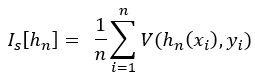
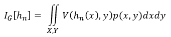
V is defined as our loss function, h_n is our classifier trained on n training samples. x is the input, for example, binary files, and y is the label, for example, clean/malicious.

Training error can be calculated by averaging the loss function over the training samples:

Generalization error is calculated by taking the expectation of the loss function over the entire input distribution:

Generalization gap or sampling error is calculated as the difference between training and generalization error:

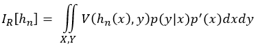
Given that for covariate shift p(y|x) is constant and p(x) changes to a new distribution p’(x), we can rewrite I_G[h_n] to create a “new-distribution error”:

Given that for covariate shift p(y|x) is constant and p(x) changes to a new distribution p'(x) , we can rewrite I_G[h_n] to create a “new-distribution error”:

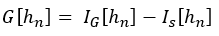
Generalization gap is formulated as the difference between training and generalization error, so it may also be helpful to express a distribution gap as the difference between I_R[h_n] and generalization error. This difference can be calculated with simple subtraction like in https://arxiv.org/abs/1902.10811 (but reversed for consistency): I_R[h_n]-I_G[h_n]. If the new distribution is harder to classify, then the gap is positive; if it is easier, the gap is negative, and if it’s the same difficulty, the gap is 0. A significant difference between the distribution gap and generalization gap is that the generalization gap is always positive, but with a new distribution, it may be that all the samples are in ‘easy’ regions for the classifier. Because training error is optimistically biased, it is very likely for training data to be in the ‘easy’ region for a classifier trained on it, keeping the generalization gap greater than or equal to 0.

Generalization gap is formulated as the difference between training and generalization error, so it may also be helpful to express a distribution gap as the difference between I_R[h_n] and generalization error. This difference can be calculated with simple subtraction like in https://arxiv.org/abs/1902.10811 (but reversed for consistency): I_R[h_n]-I_G[h_n] . If the new distribution is harder to classify, then the gap is positive; if it is easier, the gap is negative, and if it's the same difficulty, the gap is 0. A significant difference between the distribution gap and generalization gap is that the generalization gap is always positive, but with a new distribution, it may be that all the samples are in 'easy' regions for the classifier. Because training error is optimistically biased, it is very likely for training data to be in the 'easy' region for a classifier trained on it, keeping the generalization gap greater than or equal to 0.

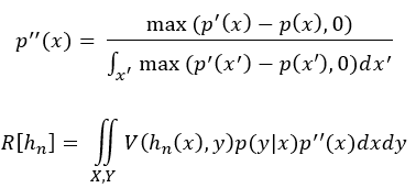
If the distributions aren’t significantly different, it may be informative to examine samples that are likely in the new distribution but unlikely in the original to provide a better test of robustness to changes in the input distribution. This next part is very informal, but one approach could be to change p’(x) to remove probability mass from areas that are likely under p(x) so that we are only evaluating samples that are more likely under p’(x) than p(x). This approach gives an error that is more focused on the samples that have become more likely in the new distribution. Here’s a pdf p’’ that subtracts p(x) from p’(x) (max prevents negative probability density, and the denominator keeps the total area at 1)

If the distributions aren't significantly different, it may be informative to examine samples that are likely in the new distribution but unlikely in the original to provide a better test of robustness to changes in the input distribution. This next part is very informal, but one approach could be to change p'(x) to remove probability mass from areas that are likely under p(x) so that we are only evaluating samples that are more likely under p'(x) than p(x) . This approach gives an error that is more focused on the samples that have become more likely in the new distribution. Here's a pdf p'' that subtracts p(x) from p'(x) (max prevents negative probability density, and the denominator keeps the total area at 1)

This equation may not be intractable, but my assumption would be using a new distribution test set sampled from p’(x) could help just like using an out-of-sample test set helps measure generalization error. It may take prior knowledge to confirm if a sample from p’(x) was also likely in p(x). For example, to better approximate R[h_n] rather than I_R[h_n] it may be worth focusing on the error of samples that are confirmed to be new malware families that had 0 probability in p(x). In the photo-vs-hand drawn case (from the ‘brief review of generalization’ section), it should be safe to assume that natural images of cats and dogs are rare when sampling hand-drawn images (with the exception of photorealistic rendering), so samples from p’’(x) (images of hand-drawn cats and dogs excluding those similar natural images of cats and dogs) should be similar to samples from p’(x) (images of hand-drawn cats and dogs).

This equation may not be intractable, but my assumption would be using a new distribution test set sampled from p'(x) could help just like using an out-of-sample test set helps measure generalization error. It may take prior knowledge to confirm if a sample from p'(x) was also likely in p(x) . For example, to better approximate R[h_n] rather than I_R[h_n] it may be worth focusing on the error of samples that are confirmed to be new malware families that had 0 probability in p(x) . In the photo-vs-hand drawn case (from the 'brief review of generalization' section), it should be safe to assume that natural images of cats and dogs are rare when sampling hand-drawn images (with the exception of photorealistic rendering), so samples from p''(x) (images of hand-drawn cats and dogs excluding those similar natural images of cats and dogs) should be similar to samples from p'(x) (images of hand-drawn cats and dogs) .

Why p(y|x) does not change: Uncertainty in the label (Why p(y|x) does not change: Uncertainty in the label)

Figure 9 shows a simple example of case B from the ‘Why p(y|x) does not change’ section. In this case, we have access to the entire input, but we define the label ‘eight’ to apply to anything that looks like an eight, and the label ‘three’ to apply to anything that looks like a three.

Figure 9 shows a simple example of case B from the 'Why p(y|x) does not change' section. In this case, we have access to the entire input, but we define the label 'eight' to apply to anything that looks like an eight, and the label 'three' to apply to anything that looks like a three.

Uncertainty arises because the input in the top left of figure 9 looks like both an eight and a three.

Often there is a spectrum of certainty, where examples near the middle may be more vulnerable to changing definitions, as shown in Figure 10:

Because the definition of malware is not precise, the same type of uncertainty can arise. A parallel example to Figure 10 for malware would look something like this:

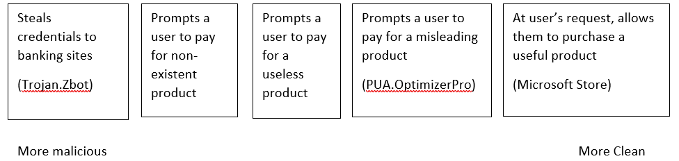
Due to uncertainty in definitions, files with behavior closer to the middle of the spectrum (sometimes called Potential Unwanted Applications or Grayware) can be more challenging to classify. Utilizing ‘soft labels’ — labels above 0 and below 1 — is one way to deal with uncertainty in the label definition.

Due to uncertainty in definitions, files with behavior closer to the middle of the spectrum (sometimes called Potential Unwanted Applications or Grayware) can be more challenging to classify. Utilizing 'soft labels' — labels above 0 and below 1 — is one way to deal with uncertainty in the label definition.

The definition of what is malicious may change, which implies a change in p(y|x). However, there are a few reasons why I think we can disregard this in practice:

The definition of what is malicious may change, which implies a change in p(y|x) . However, there are a few reasons why I think we can disregard this in practice:

1. Relating to the ‘why p(x) changes’ section, the two main causes of p(x) changing — sample selection bias and environment shift — should not change our definitions.

1. Relating to the 'why p(x) changes' section, the two main causes of p(x) changing — sample selection bias and environment shift — should not change our definitions.

2. Practically, we care most about the cases on the extreme ends of the spectrum where it is unlikely for changing definitions to have an impact. A file specifically designed to exfiltrate a user’s credit card info without their knowledge or permission will always be considered malicious, and an essential operating system file will always be considered clean. In the industry, changes in what we consider worth detecting is generally caused by debates around whether a certain behavior is clean or “potentially unwanted”

2. Practically, we care most about the cases on the extreme ends of the spectrum where it is unlikely for changing definitions to have an impact. A file specifically designed to exfiltrate a user's credit card info without their knowledge or permission will always be considered malicious, and an essential operating system file will always be considered clean. In the industry, changes in what we consider worth detecting is generally caused by debates around whether a certain behavior is clean or “potentially unwanted”

Obviously some future programs could become very difficult to classify, possibly requiring ethical philosophy to solve: for example p(y=malicious|x=code for an AGI).