贝叶斯回归线性回归区别_贝叶斯时间序列线性回归的第一步-优快云博客

本文探讨了贝叶斯回归与传统线性回归的区别，主要聚焦于贝叶斯时间序列线性回归的初步概念。通过对比两者的差异，帮助读者理解在数据分析中如何选择合适的回归模型。

摘要生成于 C知道，由 DeepSeek-R1 满血版支持，前往体验 >

贝叶斯回归线性回归区别

介绍 (Introduction)

Today time series forecasting is ubiquitous, and decision-making processes in companies depend heavily on their ability to predict the future. Through a short series of articles I will present you with a possible approach to this kind of problems, combining state-space models with Bayesian statistics.

如今，时间序列预测无处不在，并且公司的决策过程在很大程度上取决于其预测未来的能力。通过简短的系列文章，我将为您提供一种将状态空间模型与贝叶斯统计量相结合的解决此类问题的方法。

In the initial articles, I will take some of the examples from the book An Introduction to State Space Time Series Analysis from Jacques J.F. Commandeur and Siem Jan Koopman [1]. It comprises a well-known introduction to the subject of state-space modeling applied to the time series domain.

在最初的文章中，我将从Jacques JF Commandeur和Siem Jan Koopman [1]所著的《状态空间时间序列分析简介 》一书中举例说明。它包括对应用于时间序列域的状态空间建模主题的知名介绍。

My contributions will be:

我的贡献是：

A very humble attempt to close the gap between these two fields in terms of introductory and intermediate materials.
在介绍和中间材料方面，非常谦虚的尝试缩小了这两个领域之间的差距。
The presentation of concepts: on the one hand, a concise (not non-existent) mathematical basis to support our theoretical understanding and, on the other hand, an implementation from scratch of the algorithms (whenever possible, avoiding “black box” libraries). In my opinion, it is the best way to make sure that we can grasp an idea.
概念的表达：一方面，提供一个简洁的(不存在的)数学基础以支持我们的理论理解；另一方面，从头开始实现一种算法(尽可能避免使用“黑匣子”库) 。我认为，这是确保我们能够掌握想法的最佳方法。
The proper implementation of the proposed models using PyMC3 as well as their interpretation and discussion
使用PyMC3正确实施建议的模型，以及它们的解释和讨论

1.线性回归 (1. Linear regression)

In classical regression analysis, it is assumed a linear relationship between a dependent variable y and a predictor variable x. The standard regression model for n observations of y (denoted by y_i for i= 1, …,n) and x (denoted by x_i for i= 1,…,n) can be written as

在经典回归分析中，假设因变量y和预测变量x之间存在线性关系。可以将y(对i = 1，…，n表示为y_i )和x (对于i = 1，…，n表示为x_i )的n个观测值的标准回归模型写为：

where the ϵ_i ∼ NID(0, σ_ϵ²) states the assumption that the residuals (or errors) ϵ are normally and independently distributed with mean equal to zero and variance equal to σ²_ϵ.

其中ϵ_i〜NID(0，σ_ϵ²)表示以下假设：残差(或误差)normally正态且独立地分布，均值等于零，方差等于σ²_ϵ。

1.1数据 (1.1 The data)

This dataset comprises the monthly number of drivers killed or seriously injured (KSI) in the UK for the period January 1969 to December 1984, and you can find it here.

该数据集包含1969年1月至1984年12月期间英国每月死亡或重伤的驾驶员数量(KSI)，您可以在此处找到。

We will be using the log number of deaths. The log transformation can be used to turn highly skewed distributions into less skewed ones. This can be valuable both to make patterns in the data more easily interpretable and to help meeting the assumptions of inferential statistics. We will see what this means later on.

我们将使用死亡记录数。可以使用对数转换将高度偏斜的分布转换为较少偏斜的分布。这对于使数据中的模式更易于解释以及帮助满足推断统计的假设都可能是有价值的。稍后我们将了解这意味着什么。

from scipy import stats
import numpy as np
import matplotlib.pyplot as plt
%matplotlib inline
import pymc3 as pm
import arviz as azy = np.log(ukdrivers)
t = np.arange(1,len(y)+1)

In our present case, the independent variable is just time.

在我们目前的情况下，自变量只是时间。

1.2经典方法 (1.2 Classical approach)

The regression model has two unknown parameters that can be estimated with the least-squares method. It returns the values of α and β that yield the lowest average quadratic error between the observed y and the predicted ŷ.

回归模型有两个未知参数，可用最小二乘法估算。它返回在观测到的y和预测的ŷ之间产生最低平均二次误差的α和β值。

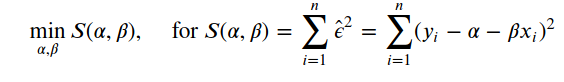
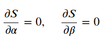
The goal is to find the values of α (hat) and β (hat) that minimize the error. For that, we take the partial derivatives for each parameter and make it equal to zero as follows,

目的是找到使误差最小的α(帽)和β(帽)的值。为此，我们将每个参数的偏导数设为零，如下所示：

After computing the equations above, we get the following

在计算了上面的等式之后，我们得到以下内容

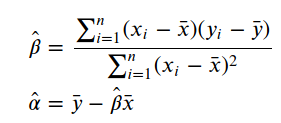
print('Least Squares\n')
β_hat = np.sum((t - t.mean())*((y - y.mean()))) / np.sum((t - t.mean())**2)
α_hat = y.mean() - β_hat*t.mean()
print("\u0302α: " + str(α_hat))
print("\u0302β: " + str(β_hat))Least Squareŝα: 7.545842731731763
̂β: -0.0014480324206279402

We can use them to plot our line of best fit.

我们可以使用它们来绘制最合适的线。

plt.plot(t, y, 'C0.')plt.plot(t, α_hat + β_hat *t, c='k',
        label=f'y = {α_hat:.4f} + {β_hat:.4f}*x')plt.ylabel('log UK drivers KSI')
plt.xlabel('Time (in months)', rotation=0)plt.legend();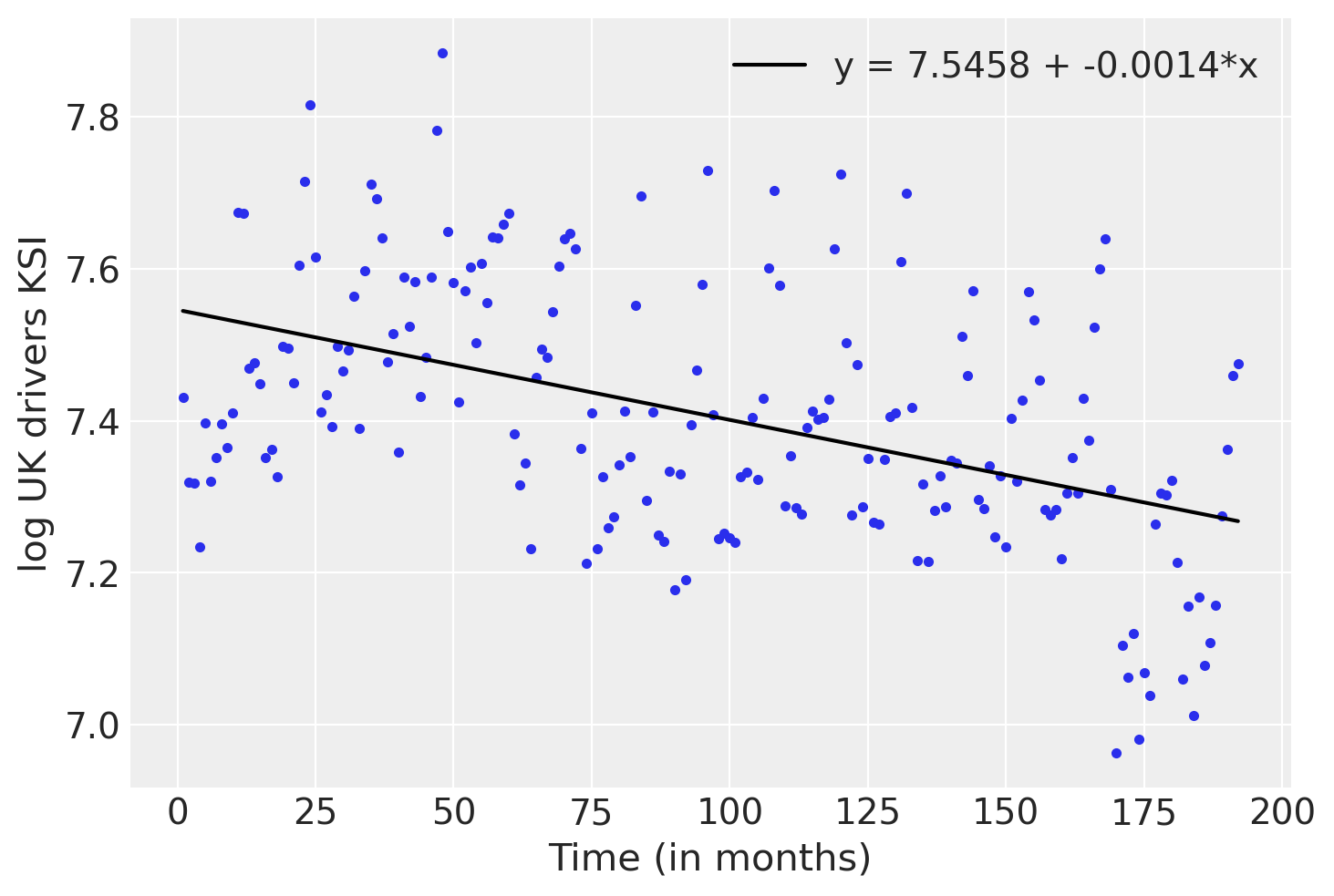

png — Regression line from the least-squares method for the log of the number of UK drivers KSI and time.

The error variance using the least-squares estimate can be calculated using

使用最小二乘估计的误差方差可以使用

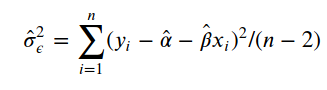
np.sum((y - α_hat - β_hat * t)**2/(len(y)-2))0.022998056021100423

2.贝叶斯方法 (2. The Bayesian way)

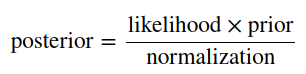
Bayes theorem without context could work as a mousetrap. Despite the relatively simple and widely known equation, there is a lot of intuition behind it. I once read that it could be seen as a lens to perceive the world. I would say that it shows a different perspective. There are useful resources to get that intuition; therefore, I will not focus too much on it. Our scope of work is on its practical aspects, making it work for our advantage. First, let’s briefly define its components.

没有上下文的贝叶斯定理可以用作捕鼠器。尽管方程式相对简单且广为人知，但背后有很多直觉。我曾经读过它可以看作是感知世界的镜头。我要说的是另一种观点。有很多有用的资源可以使人理解。因此，我不会过多地关注它。我们的工作范围是在实践方面，使它对我们有利。首先，让我们简要定义其组件。