ols回归_在幕后将ols ridge回归和pca联系起来

ols回归

引擎盖下(Under The Hood)

I am writing a new series of (relatively short) posts centered around foundational topics in statistical learning. In particular, this series will feature unexpected discoveries, less-talked-about linkages, and under-the-hood concepts for statistical learning.

我正在撰写一系列新的(相对简短的)帖子，围绕统计学习中的基础主题。 特别是，本系列文章将具有意外发现，鲜为人知的联系以及统计学习的内在概念。

My first post starts with ridge regularization, an essential concept in Data Science. Simple yet elegant relationships between ordinary least squares (OLS) estimates, ridge estimates, and PCA can be found through the lens of spectral decomposition. We see these relationships through Exercise 8.8.1 of Multivariate Analysis.

我的第一篇文章开始于岭正则化，这是数据科学中的基本概念。 普通最小二乘(OLS)估计，岭估计和PCA之间的简单而优雅的关系可以通过光谱分解的镜头找到。 我们通过多元分析练习8.8.1看到了这些关系。

This article is adapted from one of my blog posts with all the proofs omitted. If you prefer LaTex-formatted maths and HTML style pages, you can read this article on my blog.

本文改编自我的一篇博客文章，省略了所有证据。 如果您更喜欢LaTex格式的数学和HTML样式页面，则可以在我的博客上阅读此文章。

建立 (Set-up)

Given the following regression model:

给定以下回归模型：

consider the columns of X`X (In this post, ` and superscript T both means transpose) have been standardized to have mean 0 and variance 1. Then the ridge estimate of β is

考虑一下X`X的列(在这篇文章中，`和上标T均表示转置)已标准化为均值0和方差1。然后， β的岭估计为

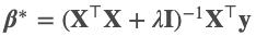
where for a given X, λ≥0 is a small fixed ridge regularization parameter. Note that when λ=0, it is just the OLS formulation. Also, consider the spectral decomposition of the var-cov matrix X`X=GLG`. Let W=XG be the principal component transformation of the original data matrix.

对于给定的X ，λ≥0是一个小的固定脊正则化参数。 注意，当λ= 0时，它只是OLS公式。 另外，考虑var-cov矩阵X`X = GLG`的频谱分解。 令W = XG是原始数据矩阵的主成分变换。

结果1.1 (Result 1.1)

If α=G`β represents the parameter vector of principal components, then we can show that the ridge estimates α* can be obtained from OLS estimates hat(α) by simply scaling them with the ridge regularization parameter:

如果α = G`β代表主要成分的参数向量，那么我们可以证明，仅通过使用ridge正则化参数对它们进行缩放，就可以从OLS估计hat( α )获得岭估计α* ：

This result shows us two important insights:

这个结果向我们展示了两个重要的见解：

1. For PC-transformed data, we can obtain the ridge estimates through a simple element-wise scaling of the OLS estimates.

   对于经过PC转换的数据，我们可以通过对OLS估计值进行简单的按元素缩放来获得岭估计值。

2. The shrinking effect of ridge regularization depends on both λ and eigenvalues of the corresponding PC:

   脊正则化的收缩效果取决于相应PC的λ和特征值：

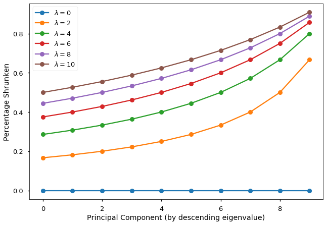
   - Larger λ corresponds to heavier shrinking for every parameter.

   -较大的λ对应于每个参数的较大收缩。

   - However, given the same λ, principal components corresponding to larger eigenvalues receive the least shrinking.

   -但是，在给定相同的λ的情况下，对应于较大特征值的主成分收缩最小。

可视化 (Visualization)

To demonstrate the two shrinking effects, I plotted the percentage shrunken (1-the ratio before hat(α)) as a function of the ordered principal components as well as the value of the ridge regularization parameter. The two shrinking effects are clearly visible from this figure.

为了演示这两个收缩效果，我绘制了收缩百分比(1- hat( α )之前的比率)与有序主成分以及脊正则化参数值的函数关系。 从该图可以清楚地看到两个收缩效果。

结果1.2 (Result 1.2)

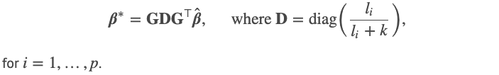
It follows from Result 1.1 that we can establish a direct link between the OLS estimate hat(β) and the ridge estimate β* through the spectral decomposition of the var-cov matrix (Hence this article’s title). Specifically, we have

从结果1.1可以得出，我们可以通过var-cov矩阵的频谱分解在OLS估计hat( β )和岭估计β*之间建立直接链接(因此，本文标题)。 具体来说，我们有

结果1.3(Result 1.3)

One measure of the quality of the estimators β* is the trace mean square error (MSE):

估计量β*的质量的一种度量是迹线均方误差(MSE)：

Now, from the previous two results, we can show that the trace MSE of the ridge estimates can be decomposed into two parts: variance and bias, and obtain an explicit formula for them. The availability of the exact formula for MSE allows things like regularization path to be computed easily. Specifically, we have

现在，从前两个结果可以看出，岭估计的迹线MSE可以分解为两部分：方差和偏差，并为其找到一个明确的公式。 MSE精确公式的可用性使诸如正则化路径之类的事情易于计算。 具体来说，我们有

where the first component is the sum of variances:

其中第一个成分是方差之和：

and the second component is the sum of squared biases:

第二部分是偏差平方的总和：

结果1.4 (Result 1.4)

This is a quick but revealing result that follows from Result 1.3. Taking a partial derivative of the trace MSE function with respect to λ and take λ=0, we get

这是从结果1.3中快速得出的结果。 取轨迹MSE函数相对于λ的偏导数，取λ= 0，我们得到

Notice that the gradient of the trace MSE function is negative when λ is 0. This tells us two things:

请注意，当λ为0时，跟踪MSE函数的梯度为负。这告诉我们两件事：

1. We can reduce the trace MSE by taking a non-zero λ value. In particular, we are trading a bit of bias for a reduction in variance as the variance function is monotonically decreasing in λ. However, we need to find the right balance between variance and bias so that the overall trace MSE is minimized.

   我们可以通过采用非零的λ值来减少跟踪MSE。 尤其是，由于方差函数单调递减λ，我们为减少方差交易了一些偏差。 但是，我们需要在方差和偏差之间找到正确的平衡，以使总迹线MSE最小化。

2. The reduction in trace MSE by ridge regularization is higher when some eigenvalues (l_i) are small. That is, when there is considerable collinearity among the predictors, ridge regularization can achieve much smaller trace MSE than OLS.

   当某些特征值(l_i)较小时，通过脊正则化对跟踪MSE的降低会更高。 也就是说，当预测变量之间存在相当大的共线性时，与OLS相比，峰正则化可以获得的跟踪MSE小得多。

可视化 (Visualization)

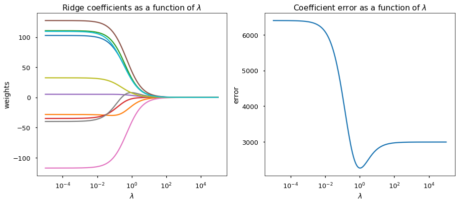
Using the sklearn.metrics.make_regression function, I generated a noisy regression data set with 50 samples and 10 features. In particular, I required that most of the variances (in PCA sense) are explained by only 5 of those 10 features, i.e. last 5 eigenvalues are relatively small. Here are the regularization path and the coefficient error plot.

使用sklearn.metrics.make_regression函数，我生成了一个包含50个样本和10个特征的嘈杂的回归数据集。 特别是，我要求大多数方差(在PCA意义上)只能由这10个特征中的5个来解释，即最后5个特征值相对较小。 这是正则化路径和系数误差图。

From the figure, we can clearly see that:

从图中可以清楚地看到：

1. Increasing λ shrinks every coefficient towards 0.
   增大λ会将每个系数缩小为0。
2. OLS procedure (left-hand side of both figures) produces erroneous (and with a large variance) estimate. the estimator MSE is significantly larger than that of the ridge regression.
   OLS程序(两个图的左侧)会产生错误的估计(且差异很大)。 估计器MSE明显大于岭回归的估计器。
3. An optimal λ is found at around 1 where the MSE of ridge estimated coefficients is minimized.
   在大约1处找到最佳λ，在该处脊估计系数的MSE最小。

4. On the other hand, λ values larger and smaller than 1 are suboptimal as they lead to over-regularization and under-regularization in this case.

   另一方面，大于和小于1的λ值不理想，因为在这种情况下，它们会导致正则化和正则化不足。

Script to plot the figure is attached below.

下面是绘制图形的脚本。

概要 (Summary)

Through the lens of spectral decomposition, we see that there is a simple yet elegant link between linear regression estimates, ridge regression estimates, and PCA. In particular:

通过频谱分解的镜头，我们看到线性回归估计，岭回归估计和PCA之间存在简单而优雅的联系。 特别是：

1. Result 1.2 says that when you have the spectral decomposition of the data var-cov matrix and the usual linear regression estimate, you can obtain the ridge estimate of every ridge regularization parameter value through a simple matrix computation. We just avoided a lot of matrix inversions there!
   结果1.2表示，当您对数据var-cov矩阵进行频谱分解并使用通常的线性回归估计时，可以通过简单的矩阵计算来获得每个脊正则化参数值的脊估计。 我们只是在那里避免了很多矩阵求逆！
2. We conducted a bias-variance decomposition for the trace MSE of the ridge estimator. It becomes evident that we could always reduce the variance of the estimators by increasing the regularization strength.
   我们对岭估计器的迹线MSE进行了偏差方差分解。 显而易见的是，我们总是可以通过增加正则化强度来减少估计量的方差。
3. While the gradient of the trace MSE function at λ=0 is negative, our visualization above suggests that the value of λ needs to be chosen carefully as it might lead to over-regularization or under-regularization.
   尽管示踪MSE函数在λ= 0处的梯度为负，但我们上面的可视化表明，需要谨慎选择λ的值，因为它可能导致过度规则化或过度规则化。

Thank you for reading this article! If you are interested in learning more about statistical learning or data science in general, you can check out some of my other writings below. Enjoy!

感谢您阅读本文！ 如果您有兴趣总体上了解更多有关统计学习或数据科学的知识，则可以在下面查看我的其他一些著作。 请享用！

翻译自: https://towardsdatascience.com/under-the-hood-what-links-ols-ridge-regression-and-pca-b64fcaf37b33

ols回归