内容损失 对抗损失_最强大的损失功能

内容损失 对抗损失

Recently, I came across the amazing paper presented in CVPR 2019 by Jon Barron about developing a robust and adaptive loss function for Machine Learning problems. This post is a review of that paper along with some necessary concepts and, it will also contain an implementation of the loss function on a simple regression problem.

最近，我遇到了乔恩·巴伦 ( Jon Barron)在CVPR 2019上发表的有关开发针对机器学习问题的健壮和自适应损失函数的惊人论文 。 这篇文章是对该论文的评论以及一些必要的概念，并且还将包含一个简单回归问题的损失函数的实现。

离群值和稳健损失的问题： (Problem with Outliers and Robust Loss:)

Consider one of the most used errors in machine learning problems- Mean Squared Error (MSE). As you know it is of the form (y-x)². One of the key characteristics of the MSE is that its high sensitivity towards large errors compared to small ones. A model trained with MSE will be biased towards reducing the largest errors. For example, a single error of 3 units will be given same importance to 9 errors of 1 unit.

考虑一下机器学习问题中最常用的错误之一-均方误差(MSE)。 如您所知，它的形式为(yx)²。 MSE的主要特征之一是与小错误相比，它对大错误的敏感性高。 用MSE训练的模型将倾向于减少最大的误差 。 例如，3个单位的单个误差将与1个单位的9个误差具有相同的重要性。

I created an example using Scikit-Learn to demonstrate how the fit varies in a simple data-set with and without taking the effect of outliers.

我使用Scikit-Learn创建了一个示例，以演示在有和没有受到异常值影响的情况下，拟合如何在简单数据集中变化。

Fig. 1: MSE and effect of outliers. (Image by Author)

图1：MSE和异常值的影响。 (图片由作者提供)

As you can see the fit line including the outliers get heavily influenced by the outliers but, the optimization problem should require the model to get more influenced by the inliers. At this point you can already think about Mean Absolute Error (MAE) as better choice than MSE, due to less sensitivity to large errors. There are various types of robust losses (like MAE) and for a particular problem we may need to test various losses. Wouldn’t it be amazing to test various loss functions on the fly while training a network? The main idea of the paper is to introduce a generalized loss function where the robustness of the loss function can be varied and, this hyperparameter can be trained while training the network, to improve performance. It is way less time consuming than finding the best loss say, by performing grid-search cross-validation. Let’s get started with the definition below —

如您所见，包括异常值在内的拟合线受到异常值的严重影响，但是，优化问题应要求模型受到较大范围的影响。 此时，由于对大误差的敏感性较低，因此您已经可以将平均绝对误差(MAE)视为比MSE更好的选择。 健壮损耗有多种类型(例如MAE)，对于特定问题，我们可能需要测试各种损耗。 在训练网络时动态地测试各种损失功能会不会令人惊讶？ 本文的主要思想是引入广义损失函数，其中损失函数的健壮性可以改变，并且可以在训练网络的同时训练该超参数，以提高性能。 通过执行网格搜索交叉验证，与找到最佳损失相比，它节省了很多时间。 让我们开始下面的定义-

稳健和适应性损失：一般形式： (Robust and Adaptive Loss: General Form:)

The general form of the robust and adaptive loss is as below —

鲁棒性和自适应性损失的一般形式如下：

Exp. 1: Robust Loss: α is the hyperparameter that controls the robustness.

经验 1：稳健性损失：α是控制稳健性的超参数。

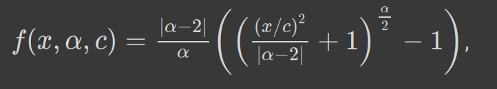
α controls the robustness of the loss function. c can be considered as a scale parameter which controls the size of the bowl near x=0. Since α acts as hyperparameter, we can see that for different values of α the loss function takes familiar forms. Let’s see below —

α控制损失函数的鲁棒性。 c可以看作是比例参数，它控制碗的大小接近x = 0。 由于α充当超参数，我们可以看到，对于不同的α值，损失函数采用熟悉的形式。 让我们在下面看到-

Exp. 2: Various losses from the adaptive loss (Expression. 1) for different values of α.

经验 2：对于不同的α值，自适应损失(表达式1)产生的各种损失。

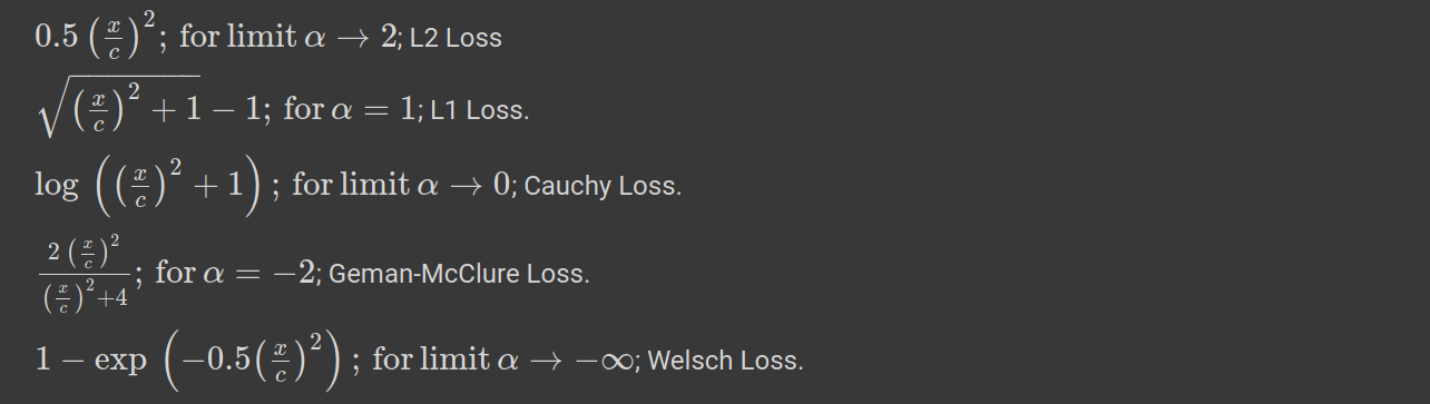
The loss function is undefined at α = 0 and 2, but taking the limit we can make approximations. From α =2 to α =1 the loss smoothly makes a transition from L2 loss to L1 loss. For different values of α we can plot the loss function to see how it behaves (fig. 2).

损失函数在α = 0和2时未定义，但是采用极限，我们可以近似。 从α = 2到α = 1，损耗平稳地从L2损耗过渡到L1损耗。 对于不同的α值，我们可以绘制损失函数以观察其行为(图2)。

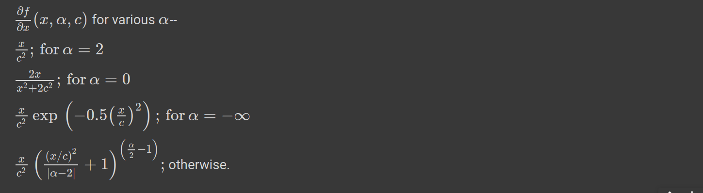
We can also spend some time with the first derivative of this loss function because the derivative is needed for gradient-based optimization. For various values of α the derivatives w.r.t x are shown below. In figure 2, I have also plotted the derivatives along with the loss function for different α.

我们也可以花一些时间处理该损失函数的一阶导数，因为基于梯度的优化需要该导数。 对于各种α值，导数wrt x如下所示。 在图2中，我还绘制了不同α的导数以及损失函数。

Exp. 3: Derivative of robust loss (Exp. 1) w.r.t x for various values of α.

经验 3：对于各种α值，稳健损耗(实验1)wrt x的导数。

自适应损耗及其导数的行为： (Behaviour of Adaptive Loss and Its Derivative:)

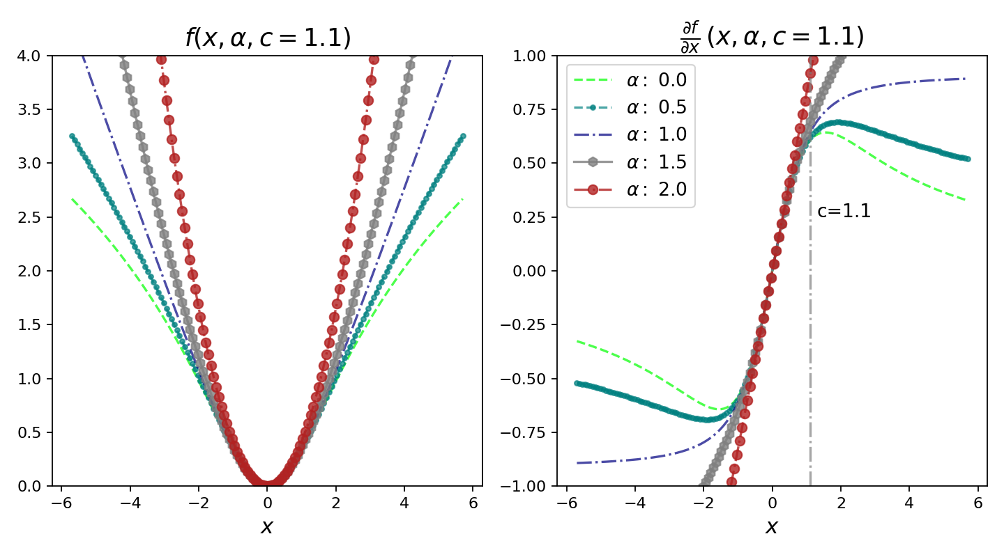
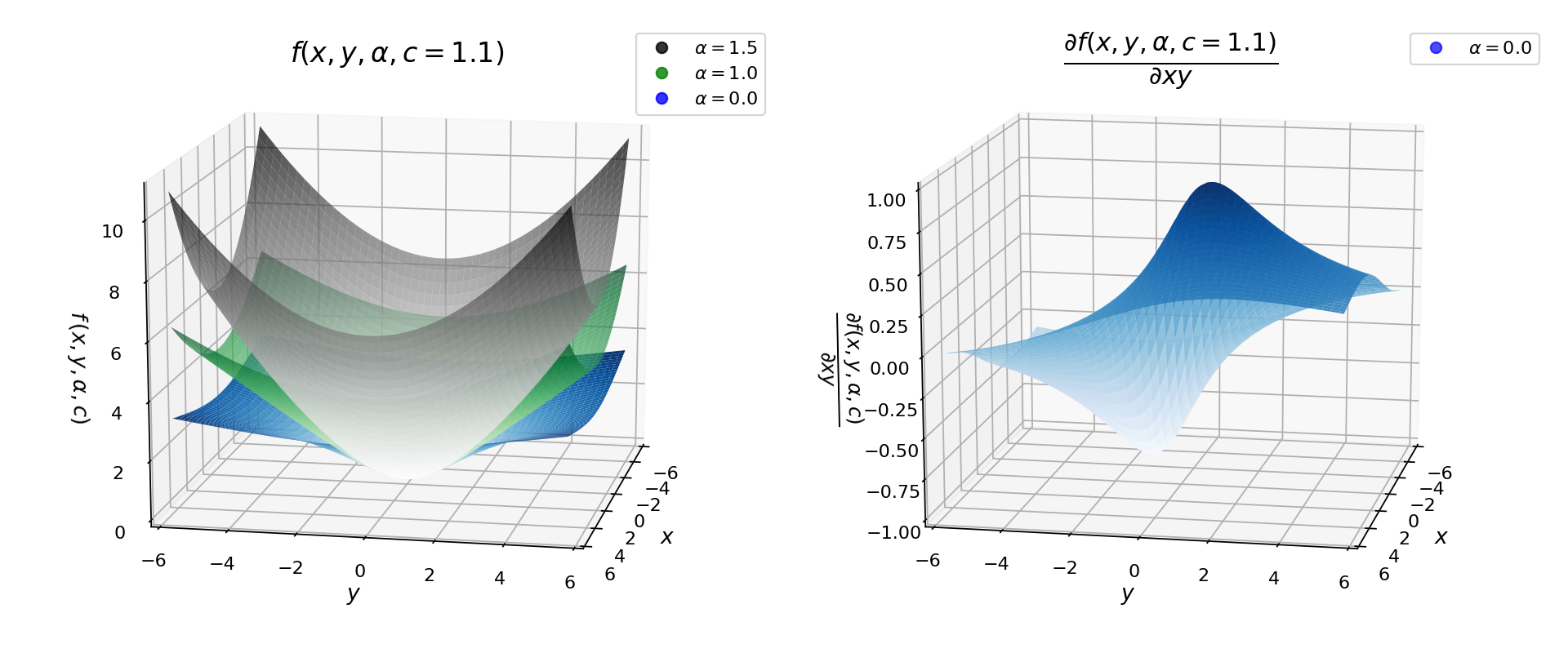
The figure below is very important to understand the behaviour of this loss function and its derivative. For the plots below, I have fixed the scale parameter c to 1.1. When x = 6.6, we can consider this as like x = 6× c. We can draw the following inferences about the loss and its derivative —

下图对于理解此损失函数及其导数的行为非常重要。 对于下面的图，我将比例参数c固定为1.1。 当x = 6.6时，我们可以将其视为x = 6× c 。 我们可以得出有关损失及其导数的以下推论-

1. The loss function is smooth for x, α and c>0 and thus suited for gradient based optimization.

   对于x，α和c > 0， 损失函数是平滑的，因此适合基于梯度的优化。

2. The loss is always zero at origin and increases monotonically for |x|>0. Monotonic nature of the loss can also be compared with taking log of a loss.

   损耗在原点处始终为零，并且对于| x |> 0单调增加 。 损失的单调性也可以与损失的对数进行比较。

3. The loss is also monotonically increasing with increasing α. This property is important for the robust nature of loss function because we can start with a higher value of α and then gradually reduce (smoothly) during optimization to enable robust estimation avoiding local minima.

   损耗也随着α的增加而单调增加。 该属性对于损失函数的鲁棒性很重要，因为我们可以从较高的α值开始，然后在优化过程中逐渐减小(平滑)以实现鲁棒的估计，从而避免局部最小值 。

4. We see that when |x|<c, the derivatives are almost linear for different values of α. This implies that the derivatives are proportional to residual’s magnitude when they are small.

   我们看到，当| x | < c ，对于不同的α值，导数几乎是线性的。 这意味着，当导数较小时，它们与残差的大小成正比 。

5. For α = 2 the derivative is throughout proportional to the residual’s magnitude. This is in general the property of MSE (L2) loss.

   对于α = 2，导数始终与残差的大小成比例。 通常，这是MSE(L2)损失的属性。

6. For α = 1 (gives us L1 Loss), we see that the derivative’s magnitude saturates to a constant value (exactly 1/c) beyond |x|>c. This implies that effect of residuals never exceeds a fixed amount.

   对于α = 1(给我们L1损失)，我们看到导数的大小饱和到一个恒定值(恰好是1 / c )，超过|。 x |> c 。 这意味着残差的影响永远不会超过固定量。

7. For α < 1, the derivative’s magnitude decreases as |x|>c. This implies that when residual increases it has less effect on the gradient, thus the outliers will have less effect during gradient descent.

   当α <1时，导数的幅度减小为| |。 x |> c 。 这意味着当残差增加时，它对梯度的影响较小，因此异常值在梯度下降期间的影响较小。

Fig. 2: Loss function and derivative of loss function as a function of α. (Image by Author)

图2：损失函数和损失函数的导数随α的变化。 (图片由作者提供)

I have also plotted below the surface plots of robust loss and its derivative for different values of α.

我还绘制了鲁棒损耗及其对于不同α值的导数的表面图。

Fig. 3: Surface plots of Adaptive Loss Function (left) and its derivative (right). (Image by Author)

图3：自适应损失函数(左)及其导数(右)的曲面图。 (图片由作者提供)

实现稳健的损失：Pytorch和Google Colab： (Implementing Robust Loss: Pytorch and Google Colab:)

Since we have gone through the basics and properties of the robust and adaptive loss function, let us put this into action. Codes used below are just slightly modified from what can be found in Jon Barron’s GitHub repository. I have also created an animation to depict how the adaptive loss finds the best-fit line as the number of iteration increases.

由于我们已经研究了健壮和自适应损失函数的基本知识和属性，因此让我们付诸实践。 下面使用的代码与Jon Barron的GitHub存储库中的代码稍作修改。 我还创建了一个动画来描述随着迭代次数的增加，自适应损失如何找到最佳拟合线。

Rather than cloning the repository and working with it, we can install it locally using pip in Colab.

无需克隆存储库并使用它，我们可以在Colab中使用pip在本地安装它。

!pip install git+https://github.com/jonbarron/robust_loss_pytorchimport robust_loss_pytorch 

We create a simple linear dataset including normally distributed noise and also outliers. Since the library uses pytorch, we convert the numpy arrays of x, y to tensors using torch.

我们创建一个简单的线性数据集，其中包括正态分布的噪声以及离群值。 由于该库使用pytorch ，我们使用torch将x，y的numpy数组转换为张量。

import numpy as np
import torch scale_true = 0.7
shift_true = 0.15x = np.random.uniform(size=n)y = scale_true * x + shift_truey = y + np.random.normal(scale=0.025, size=n) # add noise flip_mask = np.random.uniform(size=n) > 0.9 y = np.where(flip_mask, 0.05 + 0.4 * (1. — np.sign(y — 0.5)), y) 
# include outliersx = torch.Tensor(x)
y = torch.Tensor(y)

Next we define a Linear regression class using pytorch modules as below-

接下来，我们使用pytorch模块定义线性回归类，如下所示：

class RegressionModel(torch.nn.Module):   def __init__(self):      super(RegressionModel, self).__init__()      self.linear = torch.nn.Linear(1, 1) 
      ## applies the linear transformation.   def forward(self, x):      return self.linear(x[:,None])[:,0] # returns the forward pass

Next, we fit a linear regression model to our data but, first the general form of the loss function is used. Here we use a fixed value of α (α = 2.0) and it remains constant throughout the optimization procedure. As we have seen for α = 2.0 the loss function replicates L2 loss and this as we know is not optimal for problems including outliers. For optimization we use the Adam optimizer with a learning rate of 0.01.

接下来，我们将线性回归模型拟合到我们的数据，但首先使用损失函数的一般形式。 在这里，我们使用固定值α ( α = 2.0)，并且在整个优化过程中保持不变。 如我们所见，对于α = 2.0，损失函数复制了L2损失，并且我们知道，这对于包括异常值在内的问题不是最佳的。 对于优化，我们使用学习率为0.01的Adam优化器。

regression = RegressionModel()
params = regression.parameters()
optimizer = torch.optim.Adam(params, lr = 0.01)for epoch in range(2000):
   y_i = regression(x)
   # Use general loss to compute MSE, fixed alpha, fixed scale.   loss = torch.mean(robust_loss_pytorch.general.lossfun(
     y_i — y, alpha=torch.Tensor([2.]), scale=torch.Tensor([0.1])))   optimizer.zero_grad()   loss.backward()   optimizer.step()

Using the general form of the robust loss function and a fixed value of α, we can obtain the fit line. The original data, true line (line with the same slope and bias used to generate data-points excluding the outliers) and fit line are plotted below in fig. 4.

使用鲁棒损失函数的一般形式和固定值α ，我们可以获得拟合线。 原始数据，真实线(具有与用于生成数据点的斜率和偏差相同的斜率和偏差的线，但不包括异常值 )和拟合线绘制在下面的图5中。 4。

Fig. 4: General Loss Function (Image by Author)

图4：一般损失函数(作者提供)

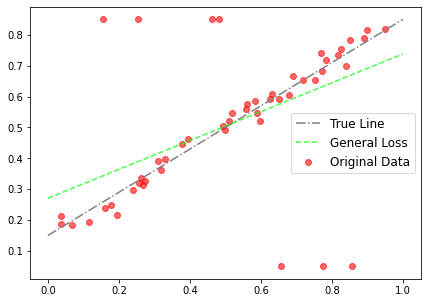
The general form of the loss function doesn’t allow α to change and thus we have to fine tune the α parameter by hand or by performing a grid-search. Also, as the figure above suggests that the fit is affected by the outliers because we used L2 loss. This is the general scenario but, what happens if we use the adaptive version of the loss function ? We call the adaptive loss module and just initialize α and let it adapt itself at each iteration step.

损失函数的一般形式不允许α改变，因此我们必须手动或通过执行网格搜索来微调α参数。 同样，如上图所示，因为我们使用了L2损失，所以拟合度受异常值的影响。 这是一般情况，但是，如果我们使用损失函数的自适应版本会怎样？ 我们称自适应损失模块，仅初始化α，并让其在每个迭代步骤中进行自适应。

regression = RegressionModel()adaptive = robust_loss_pytorch.adaptive.AdaptiveLossFunction(           num_dims = 1, float_dtype=np.float32)params = list(regression.parameters()) + list(adaptive.parameters())optimizer = torch.optim.Adam(params, lr = 0.01)for epoch in range(2000):   y_i = regression(x)   loss = torch.mean(adaptive.lossfun((y_i — y)[:,None]))
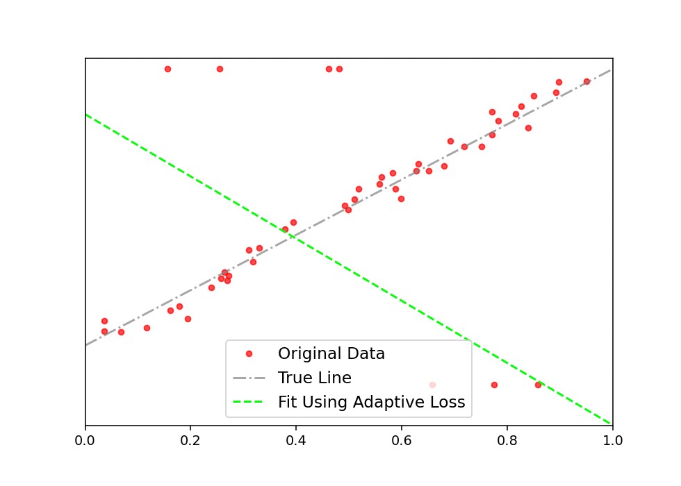
   # (y_i - y)[:, None] # numpy array or tensor   optimizer.zero_grad()   loss.backward()   optimizer.step()

Using this, and also some extra bit of code using Celluloid module, I created the animation below (figure 5). Here, you clearly see, how with increasing iterations adaptive loss finds the best fit line. This is close to the true line and it is negligibly affected by the outliers.

使用此代码以及Celluloid模块的一些额外代码，我在下面创建了动画(图5)。 在这里，您可以清楚地看到，随着迭代次数的增加，自适应损失如何找到最佳拟合线。 这接近真实界限，并且受到异常值的影响可以忽略不计。

Fig. 5: Animation of how adaptive loss function settles for the best fit. (Image by Author)

图5：自适应损失函数如何适应最佳拟合的动画。 (图片由作者提供)

讨论： (Discussion:)

We have seen how the robust loss including an hyperparameter α can be used to find the best loss-function on the fly. The paper also demonstrates how the robustness of the loss-function with α as continuous hyperparameter can be introduced to classic computer vision algorithms. Examples of implementing adaptive loss for Variational Autoencoder and Monocular depth estimations are shown in the paper and these codes are also available in Jon’s GitHub. However, the most fascinating part for me was the motivation and step by step derivation of the loss function as described in the paper. It’s easy to read so, I suggest to take a look at the paper!

我们已经看到了如何使用包括超参数α的鲁棒损耗来动态地找到最佳损耗函数。 本文还演示了如何将α作为连续超参数的损失函数的鲁棒性引入经典的计算机视觉算法中。 本文显示了为变分自动编码器和单眼深度估计实现自适应损耗的示例，这些代码也可以在Jon的GitHub中找到 。 但是，对我而言，最有趣的部分是本文所述的损失函数的动机和逐步推导。 这很容易阅读，所以我建议看一下这篇论文！

Stay strong and cheers!!

保持坚强和欢呼！！

翻译自: https://medium.com/@saptashwa/the-most-awesome-loss-function-172ffc106c99

内容损失 对抗损失