MxNet学习【1】初识

最新推荐文章于 2025-07-22 16:16:36 发布

weekdayh

最新推荐文章于 2025-07-22 16:16:36 发布

阅读量154

点赞数

CC 4.0 BY-SA版权

分类专栏： MxNet学习文章标签：神经网络

本文链接：https://blog.youkuaiyun.com/weekdayh/article/details/113795803

MxNet学习专栏收录该内容

5 篇文章

订阅专栏

MXNet学习[1] Symbol -神经网络图和自动区分

文章目录

MXNet学习[1] Symbol -神经网络图和自动区分

1.符号编程

MXNet提供了Symbol API，一个用于符号编程的接口。所谓符号编程，相比于传统的一步步计算，我们首先会定义一个计算图。计算图中包含规定的输入和输出的占位符。然后编译它，并与NDArray绑定起来进行计算。
符号编程的另一个优点是我们可以在使用它之前就优化。例如，当以指令式编程计算一个表达式时，我们不知道下一步需要什么数据。但是在符号编程里，我们已经预先定义好了需要的输出。这意味着在一边计算的时候，可以一边将中间步骤的内存回收掉。并且相同的网络下，Symbol API占用更少的内存。

2.Symbol基本组成

2.1.基础运算符

这个例子创建了一个简单的表达式：a+b。首先，使用mx.sym.Variable创建两个占位符，并命名为a和b。然后，用+运算符得到期望的Symbol。我们并不一定需要为变量命名，MXNet会自动给它生成一个独一无二的名字。比如例子中的c。

import mxnet as mx
a = mx.sym.Variable('a')
b = mx.sym.Variable('b')
c = a + b

大部分支持NDArray的运算符也支持Symbol，比如

# elemental wise multiplication
d = a * b
# matrix multiplication
e = mx.sym.dot(a, b)
# reshape
f = mx.sym.reshape(d+e, shape=(1,4))
# broadcast
g = mx.sym.broadcast_to(f, shape=(2,4))
# plot
mx.viz.plot_network(symbol=g)

上面的计算可以使用**bind()**方法绑定输入数据来执行运算.

2.2.基础神经网络

Symbol支持大量的神经网络层，这个例子构造了一个2层全连接网络，在给定输入数据格式后将其可视化。

net = mx.sym.Variable('data')
net = mx.sym.FullyConnected(data=net, name='fc1', num_hidden=128)
net = mx.sym.Activation(data=net, name='relu1', act_type="relu")
net = mx.sym.FullyConnected(data=net, name='fc2', num_hidden=10)
net = mx.sym.SoftmaxOutput(data=net, name='out')
mx.viz.plot_network(net, shape={'data':(100,200)}).view()

在这里插入图片描述

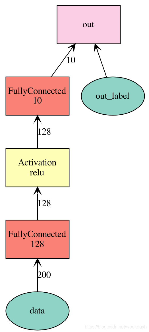
每一个symbol有一个唯一的名字。NDArray和Symbol都表示一个单独的张量。运算符表示张量之间的计算。运算符把Symbol（或NDArray）作为输入，并且接受其他超参数比如隐藏神经元个数或者激活函数，最后产生输出。我们可以把Symbol视为带有参数的函数，通过下面的方法获得这些参数：

net.list_arguments()
['data', 'fc1_weight', 'fc1_bias', 'fc2_weight', 'fc2_bias', 'out_label']
# data：变量data表示的输入数据
# fc1_weight和fc1_bias：第1个全连接网络层的权重和偏置
# fc2_weight和fc2_bias：第2个全连接网络层的权重和偏置
# out_label：损失(函数)所需要的标签

我们也可以单独给某个变量命名：

net = mx.symbol.Variable('data')
w = mx.symbol.Variable('myweight')
net = mx.symbol.FullyConnected(data=net, weight=w, name='fc1', num_hidden=128)
net.list_arguments()
['data', 'myweight', 'fc1_bias']

上面的例子中，FullyConnected层包括3个输入：data，weight，bias。当任何一个输入没有被指定时，都会得到一个自动生成的变量，这里由于指定了全连接层的权重的名称，所以输出的是myweight，而不是fc1_weight。

3、复杂的网络

MXNet提供优化好的深度学习中常用的网络Symbol。我们还可以用python自定义运算符。下面的例子先把两个symbol按元素相加，然后放入全连接网络运算符。

lhs = mx.symbol.Variable('data1')
rhs = mx.symbol.Variable('data2')
net = mx.symbol.FullyConnected(data=lhs + rhs, name='fc1', num_hidden=128)
net.list_arguments()	# ['data1', 'data2', 'fc1_weight', 'fc1_bias']

对比上面提到的单向组合，我们可以使用更灵活的方式生成Symbol。

net1 = mx.symbol.Variable('data')
net1 = mx.symbol.FullyConnected(data=net1, name='fc1', num_hidden=10)
print(net1.list_arguments())	#  ['data', 'fc1_weight', 'fc1_bias']
net2 = mx.symbol.Variable('data2')
net2 = mx.symbol.FullyConnected(data=net2, name='fc2', num_hidden=10)
print(net2.list_arguments())	#  ['data', 'fc1_weight', 'fc1_bias']

composed_net = net1(data=net2, name='composed')
print(composed_net.list_arguments()) # ['data2', 'fc2_weight', 'fc2_bias', 'fc1_weight', 'fc1_bias']

composed_net = net2(data=net1, name='composed')
print(composed_net.list_arguments())		# 报错：Symbol.ComposeKeyword argument name data not found.

这个例子中，net1作为一个函数，接收net2作为输入，得到一个组合 Symbol，这个Symbol包含net1和net2的所有属性。奇怪的是，若是以net2作为函数，net1作为输入就会报错。
当你准备构建比较大的网络时，你可能需要用一个统一的前缀命名symbols，来更好的描述网络结构。你可以使用前缀命名管理器：

data = mx.sym.Variable("data")
net = data
n_layer = 2
for i in range(n_layer):
    with mx.name.Prefix("layer%d_" % (i + 1)):
        net = mx.sym.FullyConnected(data=net, name="fc", num_hidden=100)
net.list_arguments()
['data','layer1_fc_weight','layer1_fc_bias','layer2_fc_weight','layer2_fc_bias']

3.1.深度神经网络的模块化构造

一层一层地构建一个深度神经网络（比如google inception）是很乏味的，因为网络层次太多了。所以，我们通常模块化这些构造方法。

比如，在Google Inception网络里，我们先定义一个工厂方法，把卷积核，批标准化和线性整流函数（Relu）连在一起。

def ConvFactory(data, num_filter, kernel, stride=(1,1), pad=(0, 0),name=None, suffix=''):
    conv = mx.sym.Convolution(data=data, num_filter=num_filter, kernel=kernel,
                  stride=stride, pad=pad, name='conv_%s%s' %(name, suffix))
    bn = mx.sym.BatchNorm(data=conv, name='bn_%s%s' %(name, suffix))
    act = mx.sym.Activation(data=bn, act_type='relu', name='relu_%s%s'
                  %(name, suffix))
    return act
prev = mx.sym.Variable(name="Previous Output")
conv_comp = ConvFactory(data=prev, num_filter=64, kernel=(7,7), stride=(2, 2))
shape = {"Previous Output" : (128, 3, 28, 28)}
mx.viz.plot_network(symbol=conv_comp, shape=shape)

然后我们再利用刚才的工厂方法定义一个inception模块:

def InceptionFactoryA(data, num_1x1, num_3x3red, num_3x3, num_d3x3red, num_d3x3,
                      pool, proj, name):
    # 1x1
    c1x1 = ConvFactory(data=data, num_filter=num_1x1, kernel=(1, 1), name=('%s_1x1' % name))
    # 3x3 reduce + 3x3
    c3x3r = ConvFactory(data=data, num_filter=num_3x3red, kernel=(1, 1), name=('%s_3x3' % name), suffix='_reduce')
    c3x3 = ConvFactory(data=c3x3r, num_filter=num_3x3, kernel=(3, 3), pad=(1, 1), name=('%s_3x3' % name))
    # double 3x3 reduce + double 3x3
    cd3x3r = ConvFactory(data=data, num_filter=num_d3x3red, kernel=(1, 1), name=('%s_double_3x3' % name), suffix='_reduce')
    cd3x3 = ConvFactory(data=cd3x3r, num_filter=num_d3x3, kernel=(3, 3), pad=(1, 1), name=('%s_double_3x3_0' % name))
    cd3x3 = ConvFactory(data=cd3x3, num_filter=num_d3x3, kernel=(3, 3), pad=(1, 1), name=('%s_double_3x3_1' % name))
    # pool + proj
    pooling = mx.sym.Pooling(data=data, kernel=(3, 3), stride=(1, 1), pad=(1, 1), pool_type=pool, name=('%s_pool_%s_pool' % (pool, name)))
    cproj = ConvFactory(data=pooling, num_filter=proj, kernel=(1, 1), name=('%s_proj' %  name))
    # concat
    concat = mx.sym.Concat(*[c1x1, c3x3, cd3x3, cproj], name='ch_concat_%s_chconcat' % name)
    return concat
prev = mx.sym.Variable(name="Previous Output")
in3a = InceptionFactoryA(prev, 64, 64, 64, 64, 96, "avg", 32, name="in3a")
mx.viz.plot_network(symbol=in3a, shape=shape)

最后，我们组合不同的inception模块构成整个网络。

3.2.聚合多个Symbol

为了构造含有多个损失层的神经网络，我们可以使用mxnet.sym.Group把多个Symbol聚合在一起，下面的例子聚合两个输出：

net = mx.sym.Variable('data')
fc1 = mx.sym.FullyConnected(data=net, name='fc1', num_hidden=128)
net = mx.sym.Activation(data=fc1, name='relu1', act_type="relu")
out1 = mx.sym.SoftmaxOutput(data=net, name='softmax')
out2 = mx.sym.LinearRegressionOutput(data=net, name='regression')
group = mx.sym.Group([out1, out2])
group.list_outputs()	# ['softmax_output', 'regression_output']

4.Symbol操作

Symbol和NDArray一个重要的区别是Symbol要先定义计算图然后绑定数据最后运算。这部分，我们介绍直接操作Symbol的方法。注意的是，大部分方法都位于module包。

4.1.list_arguments ()与list_outputs()

list_arguments ：给出当前符号d的输入变量的名字
list_outputs：给出符号d的输出变量的名字

import mxnet as mx
a = mx.sym.Variable("A") # represent a placeholder. These can be inputs, weights, or anything else.
b = mx.sym.Variable("B")
c = (a + b) / 10
d = c + 1
# 调用list_arguments 得到的一定就是用于d计算的所有symbol
d.list_arguments()	# ['A', 'B']

# 调用list_outputs()得到的就是输出的名字：
d.list_outputs()
# ['_plusscalar0_output'] This is the default name from adding to scalar.，

4.2.infer_shape()和infer_type()推断

上面在查看名称，下面教你如何查看各个层的大小。我们可以查询每一个symbol的参数、辅助状态和输出。在给定输入的shape或type时，我们还可以推断输出的shape或type，有利于内存分配。

import mxnet as mx
a = mx.sym.Variable('a')
b = mx.sym.Variable('b')
c = a + b
arg_name = c.list_arguments()  # get the names of the inputs：['a', 'b']
out_name = c.list_outputs()    # get the names of the outputs：['_plus0_output']

# infers output shape given the shape of input arguments
arg_shape, out_shape, _ = c.infer_shape(a=(2,3), b=(2,3))
print(arg_name)	# [(2, 3), (2, 3)]
print(out_name)	# [(2, 3)]

# infers output type given the type of input arguments
arg_type, out_type, _ = c.infer_type(a='float32', b='float32')
print(arg_type)	# [<class 'numpy.float32'>, <class 'numpy.float32'>]
print(out_type)	# [<class 'numpy.float32'>]

# 获取各层Symbol的name和对应的shape
{'input' : dict(zip(arg_name, arg_shape)),
 'output' : dict(zip(out_name, out_shape))}
# 获取各层Symbol的name和对应权值的类型type
{'input' : dict(zip(arg_name, arg_type)),
 'output' : dict(zip(out_name, out_type))}

4.3.绑定数据并执行

上面的Symbol c定义好了计算图，为了执行计算，我们首先需要绑定数据。我们可以使用bind方法，接收一个硬件环境和一个由变量名和NDArray数据组成的字典，返回一个执行器。这个执行器有一个forward方法执行计算，通过outputs属性得到结果。

ex = c.bind(ctx=mx.cpu(), args={'a' : mx.nd.ones([2,3]),
                                'b' : mx.nd.ones([2,3])})
ex.forward()
print('number of outputs = %d\nthe first output = \n%s' % (
           len(ex.outputs), ex.outputs[0].asnumpy()))
           
# number of outputs = 1
# the first output = 
# [[ 2.  2.  2.]
#  [ 2.  2.  2.]]

当然也可以在gpu上执行。注意：如果没有gpu，把gpu_device设为mx.cpu()。

gpu_device=mx.gpu() # Change this to mx.cpu() in absence of GPUs.

ex_gpu = c.bind(ctx=gpu_device, args={'a' : mx.nd.ones([3,4], gpu_device)*2,
                                      'b' : mx.nd.ones([3,4], gpu_device)*3})
ex_gpu.forward()
ex_gpu.outputs[0].asnumpy()

# array([[ 5.,  5.,  5.,  5.],
#        [ 5.,  5.,  5.,  5.],
#        [ 5.,  5.,  5.,  5.]], dtype=float32)

我们也可以用eval方法来计算symbol，相当于同时调用bind和forward方法。

ex = c.eval(ctx = mx.cpu(), a = mx.nd.ones([2,3]), b = mx.nd.ones([2,3]))
print('number of outputs = %d\nthe first output = \n%s' % (
            len(ex), ex[0].asnumpy()))
# number of outputs = 1
# the first output = 
# [[ 2.  2.  2.]
#  [ 2.  2.  2.]]

对于神经网络，更常见的方式是simple_bind，它会创建所有的参数列表。然后可以调用forward和backward（如果需要计算梯度的话）。

4.4.grad_req属性

4.4.1.grad_req=‘null’

在使用bing进行绑定，且不需要做反向递归时，可以使用上述的方式，设置grad_req=‘null’，说明不需要进行梯度的计算，bind完之后，还需要调用一个forward()，就可以运算整个过程。

import mxnet as mx
a = mx.sym.Variable("A") # represent a placeholder. These can be inputs, weights, or anything else.
b = mx.sym.Variable("B")
c = (a + b) / 10
d = c + 1
input_arguments = {}
input_arguments['A'] = mx.nd.ones((10, ), ctx=mx.cpu())
input_arguments['B'] = mx.nd.ones((10, ), ctx=mx.cpu())
executor = d.bind(ctx=mx.cpu(),
                  args=input_arguments, # args:指出输入的符号以及大小，以词典类型传入，this can be a list or a dictionary mapping names of inputs to NDArray
                  grad_req='null') # don't request gradients

当然，还可以通过executor，对输入的变量再次进行相关的赋值，如下所示：

import numpy as np
# The executor
executor.arg_dict
# {'A': NDArray, 'B': NDArray}

executor.arg_dict['A'][:] = np.random.rand(10,) # Note the [:]. This sets the contents of the array instead of setting the array to a new value instead of overwriting the variable.
executor.arg_dict['B'][:] = np.random.rand(10,)
executor.forward()
executor.outputs
# [NDArray]
output_value = executor.outputs[0].asnumpy()

executor.arg_dict['A']是NDArray类型，再使用executor.arg_dict['A'][:]=赋值，表示以numpy的值覆盖NDArray类型的值，类型依旧是NDArray；如果不加[:]，表示以numpy值的array类型直接覆盖，但运算的结果却仍然是以mx.nd.ones(10,)得到的。

4.4.2.grad_req=‘write’

这一部分，与上面的例子的区别在于添加了一个后向传播过程。那么就需要对grad_req = ‘write’ ,同时调用backforwad。

import mxnet as mx
a = mx.sym.Variable("A") # represent a placeholder. These can be inputs, weights, or anything else.
b = mx.sym.Variable("B")
c = (a + b) / 10
d = c + 1

# allocate space for inputs
input_arguments = {}
input_arguments['A'] = mx.nd.ones((10, ), ctx=mx.cpu())
input_arguments['B'] = mx.nd.ones((10, ), ctx=mx.cpu())
# allocate space for gradients
grad_arguments = {}
grad_arguments['A'] = mx.nd.ones((10, ), ctx=mx.cpu())
grad_arguments['B'] = mx.nd.ones((10, ), ctx=mx.cpu())

executor = d.bind(ctx=mx.cpu(),
                  args=input_arguments, # this can be a list or a dictionary mapping names of inputs to NDArray
                  args_grad=grad_arguments, # this can be a list or a dictionary mapping names of inputs to NDArray
                  grad_req='write') # instead of null, tell the executor to write gradients. This replaces the contents of grad_arguments with the gradients computed.

executor.arg_dict['A'][:] = np.random.rand(10,)
executor.arg_dict['B'][:] = np.random.rand(10,)

executor.forward()
# in this particular example, the output symbol is not a scalar or loss symbol.
# Thus taking its gradient is not possible.
# What is commonly done instead is to feed in the gradient from a future computation.
# this is essentially how backpropagation works.
out_grad = mx.nd.ones((10,), ctx=mx.cpu())
executor.backward([out_grad]) # because the graph only has one output, only one output grad is needed.

executor.grad_arrays
# [NDarray, NDArray]

在调用bind时，需要提前手动为梯度分配一个空间args_grad并且传入，同时将grad_req 设置为 write，再调用executor.forward()前向运行，再调用excutor.backward()后向运行，输出的symbol既不是一个标量，也不是loss symbol。需要手动传入梯度。
与bind 相对的是 simple_bind，他有一个好处：不需要手动分配计算的梯度空间大小,只需要为simple_bind 设定输入的大小，它会自动推断梯度所需的空间大小。更改后的代码如下：


input_shapes = {'A': (10,), 'B': (10, )}
executor = d.simple_bind(ctx=mx.cpu(),
                         grad_req='write', # instead of null, tell the executor to write gradients
                         **input_shapes)
executor.arg_dict['A'][:] = np.random.rand(10,)
executor.arg_dict['B'][:] = np.random.rand(10,)

executor.forward()
out_grad = mx.nd.ones((10,), ctx=mx.cpu())
executor.backward([out_grad])

4.5、加载和保存

本质上symbol和ndarray是一样的，它们都是张量，也都是运算符的输入/输出。我们可以用pickle序列化一个Symbol，还可以像之前的NDArray教程里说的直接调用save和load。

当序列化NDArray时，我们序列化里面的张量数据并且直接以二进制格式存储在硬盘上。但是symbol用的是图的概念，图由一系列运算符组成，且隐式地由输出symbol表示。所以，序列化symbol的时候，我们序列化输出Symbol。symbol还需要可读的json格式来序列化。可以用tojson方法转换symbol为json字符串。

print(c.tojson())
c.save('symbol-c.json')
c2 = mx.sym.load('symbol-c.json')
c.tojson() == c2.tojson()

{
  "nodes": [
    {
      "op": "null", 
      "name": "a", 
      "inputs": []
    }, 
    {
      "op": "null", 
      "name": "b", 
      "inputs": []
    }, 
    {
      "op": "elemwise_add", 
      "name": "_plus0", 
      "inputs": [[0, 0, 0], [1, 0, 0]]
    }
  ], 
  "arg_nodes": [0, 1], 
  "node_row_ptr": [0, 1, 2, 3], 
  "heads": [[2, 0, 0]], 
  "attrs": {"mxnet_version": ["int", 1100]}
}
True