Tensorflow教程（附完整代码）

• 综述 

1. TensorFlow是一个编程系统，用图来表示计算任务，描述了计算过程
2. 图中结点表示为op(operation),一个op获得0或多个tersor
3. tensor是一个多维数组，在图中表示边
4. 图必须在会话Session里启动
5. 变量需初始化tf.global_variables_initializer()
6. TensorFlow程序可以看做独立的两部分：构建计算图 与 运行计算图

1、Session

当要获取tensor值时，需要初始化一个tf.Session对象，调用Session.run()方法获取张量的值

from __future__ import print_function
import tensorflow as tf

matrix1 = tf.constant([[3, 3]])
matrix2 = tf.constant([[2],
                       [2]])
product = tf.matmul(matrix1, matrix2)  # matrix multiply np.dot(m1, m2)

# method 1
sess = tf.Session()
result = sess.run(product)
print(result)
sess.close()

# method 2
with tf.Session() as sess:
    result2 = sess.run(product)
    print(result2)

可以通过Session.run()方法运行操作或变量的值。但如果参数只有一个的话，那么可以使用eval()方法会比较简便

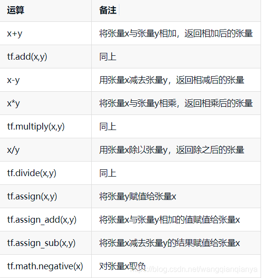
assign_add是TensorFlow中的运算函数，会将第一个参数和第二个参数的值相加后赋值给第一个参数。类似于C语言中的+=

constant = tf.constant([1, 2, 3])
tensor = constant * constant
print(tensor.eval())

p = tf.placeholder(tf.float32)
t = p + 1.0
t.eval()  # 错误！p没有初始化
t.eval(feed_dict={p:2.0})  # 正确！因为p被初始化了

#值得注意的是，不只是张量的值，操作也可以使用eval()方法，如下：
v=tf.Varibale(1)
sess=tf.Session()
sess.run(tf.global_variables_initializer())
tf.assign_add(v,tf.constant(1)).eval()
print(v.eval())

2、Constant

 tf.constant(value,dtype=None,shape=None,name='Const',verify_shape=False)

value的值可以为3、1,2,3,4,5]，[[22,32]，[32,4]]等

3、Variable

from __future__ import print_function
import tensorflow as tf

state = tf.Variable(0, name='counter')
#print(state.name)
one = tf.constant(1)

new_value = tf.add(state, one)
update = tf.assign(state, new_value)

# tf.initialize_all_variables() no long valid from
# 2017-03-02 if using tensorflow >= 0.12
if int((tf.__version__).split('.')[1]) < 12 and int((tf.__version__).split('.')[0]) < 1:
    init = tf.initialize_all_variables()
else:
    init = tf.global_variables_initializer()

with tf.Session() as sess:
    sess.run(init)
    for _ in range(3):
        sess.run(update)
        print(sess.run(state))

4、placeholder：run的时候才赋值

tf.placeholder(dtype,shape=None,name=None)

placeholder在运算时得通过Session.run()方法中的feed_dict参数获得初值

from __future__ import print_function
import tensorflow as tf

input1 = tf.placeholder(tf.float32)
input2 = tf.placeholder(tf.float32)
output = tf.multiply(input1, input2)

with tf.Session() as sess:
    print(sess.run(output, feed_dict={input1: [7.], input2: [2.]}))

5、tensor间运算 

注意：给张量赋值必须用tf.assign()系列函数，不能直接用=

6、activation function

from __future__ import print_function
import tensorflow as tf


def add_layer(inputs, in_size, out_size, activation_function=None):
    Weights = tf.Variable(tf.random_normal([in_size, out_size]))
    biases = tf.Variable(tf.zeros([1, out_size]) + 0.1)
    Wx_plus_b = tf.matmul(inputs, Weights) + biases
    if activation_function is None:#线性
        outputs = Wx_plus_b
    else:
        outputs = activation_function(Wx_plus_b)
    return outputs

6、tensorflow搭建自己的神经网络（输入输出1个神经元，隐层10个神经元） 画出

from __future__ import print_function
import tensorflow as tf
import numpy as np
import matplotlib.pyplot as plt

def add_layer(inputs, in_size, out_size, activation_function=None):
    Weights = tf.Variable(tf.random_normal([in_size, out_size]))
    biases = tf.Variable(tf.zeros([1, out_size]) + 0.1)
    Wx_plus_b = tf.matmul(inputs, Weights) + biases
    if activation_function is None:
        outputs = Wx_plus_b
    else:
        outputs = activation_function(Wx_plus_b)
    return outputs

# Make up some real data
x_data = np.linspace(-1, 1, 300)[:, np.newaxis]
noise = np.random.normal(0, 0.05, x_data.shape)
y_data = np.square(x_data) - 0.5 + noise

##plt.scatter(x_data, y_data)
##plt.show()

# define placeholder for inputs to network
xs = tf.placeholder(tf.float32, [None, 1])
ys = tf.placeholder(tf.float32, [None, 1])
# add hidden layer
l1 = add_layer(xs, 1, 10, activation_function=tf.nn.relu)
# add output layer
prediction = add_layer(l1, 10, 1, activation_function=None)

# the error between prediction and real data
loss = tf.reduce_mean(tf.reduce_sum(tf.square(ys-prediction), reduction_indices=[1]))
train_step = tf.train.GradientDescentOptimizer(0.1).minimize(loss)
# important step
sess = tf.Session()
# tf.initialize_all_variables() no long valid from
# 2017-03-02 if using tensorflow >= 0.12
if int((tf.__version__).split('.')[1]) < 12 and int((tf.__version__).split('.')[0]) < 1:
    init = tf.initialize_all_variables()
else:
    init = tf.global_variables_initializer()
sess.run(init)

# plot the real data
fig = plt.figure()
ax = fig.add_subplot(1,1,1)
ax.scatter(x_data, y_data)
plt.ion()
plt.show()


for i in range(1000):
    # training
    sess.run(train_step, feed_dict={xs: x_data, ys: y_data})
    if i % 50 == 0:
        # to visualize the result and improvement
        try:
            ax.lines.remove(lines[0])
        except Exception:
            pass
        prediction_value = sess.run(prediction, feed_dict={xs: x_data})
        # plot the prediction
        lines = ax.plot(x_data, prediction_value, 'r-', lw=5)
        plt.pause(1)

拟合多项式：3x^2+4x+5

# -*- coding: utf-8 -*-
import tensorflow as tf
import numpy as np
import matplotlib.pyplot as plt

plotdata = {"batchsize": [], "loss": []}


def moving_average(a, w=10):
    if len(a) < w:
        return a[:]
    return [val if idx < w else sum(a[(idx - w):idx]) / w for idx, val in enumerate(a)]


# 生成模拟数据
train_X = np.linspace(-1, 1, 200)
train_Y = 3 * train_X * train_X + 4 * train_X + 5 + np.random.randn(*train_X.shape) * 0.3  # y=2x，但是加入了噪声

# 显示模拟数据点
plt.plot(train_X, train_Y, 'ro', label='Original data')
plt.legend()
plt.show()
# 创建模型
# 占位符
X = tf.placeholder("float")
Y = tf.placeholder("float")
# 模型参数
W = tf.Variable([0.]*3, name="weight")

# 前向结构
terms=[]
for i in range(3):#修改3为多项式项数
    term=tf.multiply(W[i],tf.pow(X,i))
    terms.append(term)
z = tf.add_n(terms)#实现列表元素累加

# 反向优化
cost = tf.reduce_mean(tf.square(Y - z))
learning_rate = 0.01
optimizer = tf.train.GradientDescentOptimizer(learning_rate).minimize(cost)  # Gradient descent

# 初始化变量
init = tf.global_variables_initializer()
# 训练参数
training_epochs = 20
display_step = 2

# 启动session
with tf.Session() as sess:
    sess.run(init)

    # Fit all training data
    for epoch in range(training_epochs):
        for (x, y) in zip(train_X, train_Y):
            sess.run(optimizer, feed_dict={X: x, Y: y})
        print(z.dtype)
        # 显示训练中的详细信息
        if epoch % display_step == 0:
            loss = sess.run(cost, feed_dict={X: train_X, Y: train_Y})
            print("Epoch:", epoch + 1, "cost=", loss, "W=", sess.run(W))
            if not (loss == "NA"):
                plotdata["batchsize"].append(epoch)
                plotdata["loss"].append(loss)

    print(" Finished!")
    print("cost=", sess.run(cost, feed_dict={X: train_X, Y: train_Y}), "W=", sess.run(W))
    # print ("cost:",cost.eval({X: train_X, Y: train_Y}))

    # 图形显示
    plt.plot(train_X, train_Y, 'ro', label='Original data')
    plt.plot(train_X, sess.run(W[2]) * train_X* train_X+sess.run(W[1]) * train_X +sess.run(W[0]), label='Fitted line')
    plt.legend()
    plt.show()

    plotdata["avgloss"] = moving_average(plotdata["loss"])
    plt.figure(1)
    plt.subplot(211)
    plt.plot(plotdata["batchsize"], plotdata["avgloss"], 'b--')
    plt.xlabel('Minibatch number')
    plt.ylabel('Loss')
    plt.title('Minibatch run vs. Training loss')

    plt.show()

    print("x=0.2，z=", sess.run(z, feed_dict={X: 0.2}))

6、Classification

from __future__ import print_function
import tensorflow as tf
from tensorflow.examples.tutorials.mnist import input_data
# number 1 to 10 data
mnist = input_data.read_data_sets('MNIST_data', one_hot=True)

def add_layer(inputs, in_size, out_size, activation_function=None,):
    # add one more layer and return the output of this layer
    Weights = tf.Variable(tf.random_normal([in_size, out_size]))
    biases = tf.Variable(tf.zeros([1, out_size]) + 0.1,)
    Wx_plus_b = tf.matmul(inputs, Weights) + biases
    if activation_function is None:
        outputs = Wx_plus_b
    else:
        outputs = activation_function(Wx_plus_b,)
    return outputs

def compute_accuracy(v_xs, v_ys):
    global prediction
    y_pre = sess.run(prediction, feed_dict={xs: v_xs})
    correct_prediction = tf.equal(tf.argmax(y_pre,1), tf.argmax(v_ys,1))
    accuracy = tf.reduce_mean(tf.cast(correct_prediction, tf.float32))
    result = sess.run(accuracy, feed_dict={xs: v_xs, ys: v_ys})
    return result

# define placeholder for inputs to network
xs = tf.placeholder(tf.float32, [None, 784]) # 28x28
ys = tf.placeholder(tf.float32, [None, 10])

# add output layer
prediction = add_layer(xs, 784, 10,  activation_function=tf.nn.softmax)

# the error between prediction and real data
cross_entropy = tf.reduce_mean(-tf.reduce_sum(ys * tf.log(prediction),
                                              reduction_indices=[1]))       # loss
train_step = tf.train.GradientDescentOptimizer(0.5).minimize(cross_entropy)

sess = tf.Session()
# important step
# tf.initialize_all_variables() no long valid from
# 2017-03-02 if using tensorflow >= 0.12
if int((tf.__version__).split('.')[1]) < 12 and int((tf.__version__).split('.')[0]) < 1:
    init = tf.initialize_all_variables()
else:
    init = tf.global_variables_initializer()
sess.run(init)

for i in range(1000):
    batch_xs, batch_ys = mnist.train.next_batch(100)
    sess.run(train_step, feed_dict={xs: batch_xs, ys: batch_ys})
    if i % 50 == 0:
        print(compute_accuracy(
            mnist.test.images, mnist.test.labels))

过拟合解决方法：（训练误差不是越小越好）

1、增大训练数据（随着数据量的增大曲线会逐渐拉直）

2、正则化（cost在最小二乘基础上加上L1:|W| 或L2:W^2）

3、对于神经网络还可以采用dropout方法

tensorflow实现线性回归

# -*- coding: utf-8 -*-
"""
Created on Tue Jun  6 18:52:37 2017

@author: 代码医生 qq群：40016981，公众号：xiangyuejiqiren
@blog：http://blog.youkuaiyun.com/lijin6249
"""

import tensorflow as tf
import numpy as np
import matplotlib.pyplot as plt


plotdata = { "batchsize":[], "loss":[] }
def moving_average(a, w=10):
    if len(a) < w: 
        return a[:]    
    return [val if idx < w else sum(a[(idx-w):idx])/w for idx, val in enumerate(a)]


#生成模拟数据
train_X = np.linspace(-1, 1, 100)
train_Y = 2 * train_X + np.random.randn(*train_X.shape) * 0.3 # y=2x，但是加入了噪声
#显示模拟数据点
plt.plot(train_X, train_Y, 'ro', label='Original data')
plt.legend()
plt.show()




# 创建模型
# 占位符
X = tf.placeholder("float")
Y = tf.placeholder("float")
# 模型参数
W = tf.Variable(tf.random_normal([1]), name="weight")
b = tf.Variable(tf.zeros([1]), name="bias")

# 前向结构
z = tf.multiply(X, W)+ b

#反向优化
cost =tf.reduce_mean( tf.square(Y - z))
learning_rate = 0.01
optimizer = tf.train.GradientDescentOptimizer(learning_rate).minimize(cost) #Gradient descent

# 初始化变量
init = tf.global_variables_initializer()
# 训练参数
training_epochs = 20
display_step = 2

# 启动session
with tf.Session() as sess:
    sess.run(init)

    # Fit all training data
    for epoch in range(training_epochs):
        for (x, y) in zip(train_X, train_Y):
            sess.run(optimizer, feed_dict={X: x, Y: y})

        #显示训练中的详细信息
        if epoch % display_step == 0:
            loss = sess.run(cost, feed_dict={X: train_X, Y:train_Y})
            print ("Epoch:", epoch+1, "cost=", loss,"W=", sess.run(W), "b=", sess.run(b))
            if not (loss == "NA" ):
                plotdata["batchsize"].append(epoch)
                plotdata["loss"].append(loss)

    print (" Finished!")
    print ("cost=", sess.run(cost, feed_dict={X: train_X, Y: train_Y}), "W=", sess.run(W), "b=", sess.run(b))
    #print ("cost:",cost.eval({X: train_X, Y: train_Y}))

    #图形显示
    plt.plot(train_X, train_Y, 'ro', label='Original data')
    plt.plot(train_X, sess.run(W) * train_X + sess.run(b), label='Fitted line')
    plt.legend()
    plt.show()
    
    plotdata["avgloss"] = moving_average(plotdata["loss"])
    plt.figure(1)
    plt.subplot(211)
    plt.plot(plotdata["batchsize"], plotdata["avgloss"], 'b--')
    plt.xlabel('Minibatch number')
    plt.ylabel('Loss')
    plt.title('Minibatch run vs. Training loss')
     
    plt.show()

    print ("x=0.2，z=", sess.run(z, feed_dict={X: 0.2}))
    

---

代码来源：https://github.com/MorvanZhou/tutorials/tree/master/tensorflowTUT