TF-- 二 数据拟合的一般步骤

目录

一，简单的线性回归

1.数据准备

2.准备好placeholder

3.初始化参数/权重

4.计算预测结果

5.计算损失函数值

6.初始化optimizer

7.指定迭代次数，并在session里执行graph

---

一，简单的线性回归

1.数据准备

实际的数据大家可以通过pandas等package读入。

此处的数据是自己造的。

%matplotlib inline
import numpy as np
import tensorflow as tf
import matplotlib.pyplot as plt
plt.rcParams["figure.figsize"] = (14,8)

n_observations = 100
xs = np.linspace(-3, 3, n_observations)
ys = np.sin(xs) + np.random.uniform(-0.5, 0.5, n_observations)
plt.scatter(xs, ys)
plt.show()

2.准备好placeholder

X = tf.placeholder(tf.float32, name='X')
Y = tf.placeholder(tf.float32, name='Y')

3.初始化参数/权重

W = tf.Variable(tf.random_normal([1]), name='weight')
b = tf.Variable(tf.random_normal([1]), name='bias')

4.计算预测结果

Y_pred = tf.add(tf.multiply(X, W), b)

5.计算损失函数值

loss = tf.square(Y - Y_pred, name='loss')

6.初始化optimizer

learning_rate = 0.01
optimizer = tf.train.GradientDescentOptimizer(learning_rate).minimize(loss)

7.指定迭代次数，并在session里执行graph

n_samples = xs.shape[0]
with tf.Session() as sess:
	# 记得初始化所有变量
	sess.run(tf.global_variables_initializer()) 
	
	writer = tf.summary.FileWriter('./graphs/linear_reg', sess.graph)
	
	# 训练模型
	for i in range(50):
		total_loss = 0
		for x, y in zip(xs, ys):
			# 通过feed_dic把数据灌进去
			_, l = sess.run([optimizer, loss], feed_dict={X: x, Y:y}) 
			total_loss += l
		if i%5 ==0:
			print('Epoch {0}: {1}'.format(i, total_loss/n_samples))

	# 关闭writer
	writer.close() 
	
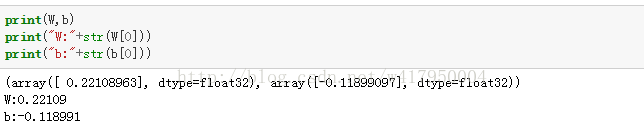
	# 取出w和b的值
	W, b = sess.run([W, b]) 

输出：

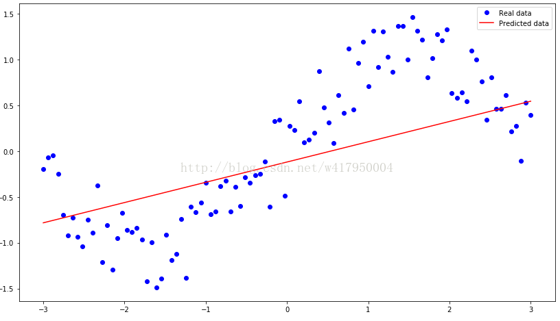
画图拟合：

plt.plot(xs, ys, 'bo', label='Real data')
plt.plot(xs, xs * W + b, 'r', label='Predicted data')
plt.legend()
plt.show()

拟合结果如下图所示：