Basic Concepts in ZhuSuan解析

地址：https://zhusuan.readthedocs.io/en/latest/tutorials/concepts.html

分布和随机传感器

概率分布是构建有向图形模型（贝叶斯网络）的关键组件。 ZhuSuan为他们提供了两层抽象：Distribution和StochasticTensor，这对初学者来说可能有点混乱。我们在这里明确他们的定义和联系。

distribution 

分布类是各种概率分布的基类，它支持批量输入，生成批量样本并评估批量给定值的概率。 

可在以下页面上找到所有可用分发的列表：

单变量分布
多变量分布

这些分布可以通过（例如，单变量正态分布）从ZhuSuan访问：

>>> import zhusuan as zs
>>> a = zs.distributions.Normal(mean=0., logstd=0.)

 分布的典型输入形状类似于batch_shape + input_shape。 其中input_shape表示非批输入参数的形状; batch_shape表示将多少独立输入馈送到分发中。 通常，分发支持广播输入。

可以通过调用分发对象的sample（）方法生成样本。 形状为（[n_samples] +）batch_shape + value_shape。 仅当传递n_samples为None（默认情况下）时，才会省略第一个附加轴，在这种情况下会生成一个样本。 value_shape是分布的非批量值形状。 对于单变量分布，其value_shape为[]。

单变量分布示例（正常）：

>>> import tensorflow as tf
>>> _ = tf.InteractiveSession()

>>> b = zs.distributions.Normal([[-1., 1.], [0., -2.]], [0., 1.])

>>> b.batch_shape.eval()
array([2, 2], dtype=int32)

>>> b.value_shape.eval()
array([], dtype=int32)

>>> tf.shape(b.sample()).eval()
array([2, 2], dtype=int32)

>>> tf.shape(b.sample(1)).eval()
array([1, 2, 2], dtype=int32)

>>> tf.shape(b.sample(10)).eval()
array([10,  2,  2], dtype=int32)

多变量分布的示例（OnehotCategorical）：

>>> c = zs.distributions.OnehotCategorical([[0., 1., -1.],
...                                         [2., 3., 4.]])

>>> c.batch_shape.eval()
array([2], dtype=int32)

>>> c.value_shape.eval()
array([3], dtype=int32)

>>> tf.shape(c.sample()).eval()
array([2, 3], dtype=int32)

>>> tf.shape(c.sample(1)).eval()
array([1, 2, 3], dtype=int32)

>>> tf.shape(c.sample(10)).eval()
array([10,  2,  3], dtype=int32)

在某些情况下，将一批随机变量分组到单个事件中，以便可以一起计算它们的概率。 这是通过设置group_ndims参数来实现的，该参数默认为0. batch_shape中的最后一个group_ndims轴数被分组为单个事件。 例如，Normal（...，group_ndims = 1）将其batch_shape的最后一个轴设置为单个事件，即具有标识协方差矩阵的多元Normal。

可以通过将给定值传递给分布对象的log_prob（）方法来评估对数概率密度（质量）函数。 在这种情况下，给定的Tensor应该可以广播到shape（... +）batch_shape + value_shape。 返回的Tensor有形状：

(... + )batch_shape[:-group_ndims]. For example:

>>> d = zs.distributions.Normal([[-1., 1.], [0., -2.]], 0.,
...                             group_ndims=1)

>>> d.log_prob(0.).eval()
array([-2.83787704, -3.83787727], dtype=float32)

>>> e = zs.distributions.Normal(tf.zeros([2, 1, 3]), 0.,
...                             group_ndims=2)

>>> tf.shape(e.log_prob(tf.zeros([5, 1, 1, 3]))).eval()
array([5, 2], dtype=int32)

StochasticTensor

而Distribution为概率分布提供了基本功能。 使用它们直接构建计算图仍然很痛苦，因为它们不知道任何内部可重用性作为贝叶斯网络中的随机节点：一旦从分布中进行采样，当您想要观察它时，就无法重用根系图。

为了应对这一挑战，ZhuSuan提供了另一种基于发行版的抽象。 这是StochasticTensor。 对于zhusuan.distributions中可用的所有分布，有一个相应的StochasticTensor，可以通过zs.Normal访问（例如，单变量Normal StochasticTensor）。 他们的列表在此页面上。

StochasticTensor只能在BayesianNet上下文中构建。 它们的实例类似Tensor，可以使用张量流基元透明地构建贝叶斯网络。 有关用法示例，请参见BayesianNet部分。

Use zs.Normal when you want StochasticTensor and use zs.distributions.Normal when you want Distribution. 

BayesianNet 

BayesianNet类是支持ZhuSuan中贝叶斯网络（定向图形模型）的模型构建的上下文类。 BayesianNet表示具有两种节点的DAG：

• 确定性节点，由任何张量流操作组成。
• 随机节点，由StochasticTensor构建。 

要启动BayesianNet内容： 

import zhusuan as zs
with zs.BayesianNet() as model:
    # build the model

 贝叶斯线性回归的例子：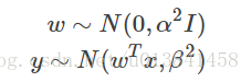

import tensorflow as tf
import zhusuan as zs

def bayesian_linear_regression(x, alpha, beta):
    with zs.BayesianNet() as model:
        w = zs.Normal('w', mean=0., logstd=tf.log(alpha)
        y_mean = tf.reduce_sum(tf.expand_dims(w, 0) * x, 1)
        y = zs.Normal('y', y_mean, tf.log(beta))
    return model

要观察网络中的任何随机节点，在构造BayesianNet时传递（name，Tensor）对的字典映射。 这将把观察值分配给相应的StochasticTensor。 例如：

def bayesian_linear_regression(observed, x, alpha, beta):
    with zs.BayesianNet(observed=observed) as model:
        w = zs.Normal('w', mean=0., logstd=tf.log(alpha)
        y_mean = tf.reduce_sum(tf.expand_dims(w, 0) * x, 1)
        y = zs.Normal('y', y_mean, tf.log(beta))
    return model

model = bayesian_linear_regression({'w': w_obs}, ...)

将设置w被观察。 结果是y_mean是根据w（w_obs）的观测值而不是w的样本计算的。 使用不同的观察参数调用上述函数可以使用不同的观察来实例化贝叶斯网络，这是概率图形模型的常见行为。

note:通过的观察必须与StochasticTensor具有相同的类型和形状。

 如果在此函数中创建了tensorflow变量，您可能希望重用它。 ZhuSuan提供了一种简单的方法。 你可以在函数中添加一个装饰器：

@zs.reuse(scope="model")
def bayesian_linear_regression(observed, x, alpha, beta):
    ...

有关详细信息，请参阅reuse（）。

构建完成后，BayesianNet支持网络查询：

# get samples of random variable y following generative process
# in the network
model.outputs('y')

# because w is observed in this case, its observed value will be
# returned
model.outputs('w')

# get local log probability values of w and y, which returns
# log p(w) and log p(y|w, x)
model.local_log_prob(['w', 'y'])

# query many quantities at the same time
model.query('w', outputs=True, local_log_prob=True)