


 这篇博客详细介绍了如何使用CaffeNet进行深度学习训练,包括创建lmdb数据集、计算均值、设置网络与求解器、训练过程以及模型的GPU使用和时间分析。此外,还讲解了如何使用CaffeNet进行特征提取和分类,并通过pycaffe进行CPU和GPU分类的比较。最后,文章探讨了CaffeNet的微调技术,包括Flickr数据集的下载、网络定义与运行、风格分类器的训练以及端到端的微调方法。
本文主要分四部分
1. 在命令行进行训练
2. 使用pycaffe进行分类及特征可视化
3. 进行微调,将caffenet使用在图片风格的预测上
1 使用caffeNet训练自己的数据集
主要参考:
官方网址:
主要步骤:
1. 准备数据集
2. 标记数据集
3. 创建lmdb格式的数据
4. 计算均值
5. 设置网络及求解器
6. 运行求解
由于imagenet的数据集太大,博主电脑显卡840m太弱,所以就选择了第二个网址中的数据集
http://pan.baidu.com/s/1o60802I
,其训练集为1000张10类图片,验证集为200张图片,原作者已经整理好其标签放于对应的txt文件中,所以这里就省去上面的1-2步骤。
1.1 创建lmdb
使用对应的数据集创建lmdb:
这里使用 examples/imagenet/create_imagenet.sh,需要更改其路径和尺寸设置的选项,为了减小更改的数目,这里并没有自己新创建一个文件夹,而是直接使用了原来的imagenet的文件夹,而且将train.txt,val.txt都放置于/data/ilsvrc12中,
TRAIN_DATA_ROOT=/home/beatree/caffe-rc3/examples/imagenet/train/
VAL_DATA_ROOT=/home/beatree/caffe-rc3/examples/imagenet/val/
RESIZE=
true
注意下面的地址的含义:
echo
"Creating train lmdb..."
GLOG_logtostderr=
1
$TOOLS
/convert_imageset \ --resize_height=
$RESIZE_HEIGHT
\ --resize_width=
$RESIZE_WIDTH
\ --shuffle \
$TRAIN_DATA_ROOT
\
$DATA
/train.txt \
$EXAMPLE
/ilsvrc12_train_lmdb
主要用了tools里的convert_imageset
1.2 计算均值
模型需要我们从每张图片减去均值,所以我们需要获得训练的均值,直接利用./examples/imagenet/make_imagenet_mean.sh创建均值文件binaryproto,如果之前创建了新的路径,这里同样需要修改sh文件里的路径。
这里的主要语句是
$TOOLS
/compute_image_mean
$EXAMPLE
/ilsvrc12_train_lmdb \
$DATA
/imagenet_mean.binaryproto
- 1
- 2
如果显示
Check failed: size_in_datum == data_size () Incorrect data field size
说明上一步的图片没有统一尺寸
1.3 设置网络及求解器
这里是利用原文的网络设置tain_val.prototxt和slover.prototext,在models/bvlc_reference_caffenet/solver.prototxt路径中,这里的训练和验证的网络基本一样用
include { phase: TRAIN } or include { phase: TEST }
和来区分,其两点不同之处具体为:
transform_param
{ mirror:
true#不同1:训练集会randomly mirrors the input image crop_size: 227 mean_file:
"data/ilsvrc12/imagenet_mean.binaryproto"
}data_param
{ source:
"examples/imagenet/ilsvrc12_train_lmdb"
#不同2:来源不同 batch_size: 32#原文很大,显卡比较弱的会内存不足,这里改为了32,这里根据需要更改,验证集和训练集的设置也不一样 backend: LMDB
}
另外在输出层也有不同,训练时的loss需要用来进行反向传递,而val就不需要了。
solver.protxt的改动:
根据
net
:
"/home/beatree/caffe-rc3/examples/imagenet/train_val.prototxt"#网络配置存放地址
test_iter
:
4, 每个批次是50,一共200个
test_interval
:
300 #每300次测试一次
base_lr
:
0.01 #是基础学习率,因为数据量小,0.01 就会下降太快了,因此可以改成 0.001,这里博主没有改
lr_policy
:
"step" #lr可以变化
gamma
:
0.1 #学习率变化的比率
stepsize
:
300
display
:
20 #20层显示一次
max_iter
:
1200 一共迭代1200次
momentum
:
0.9
weight_decay
:
0.0005
snapshot
:
600 #每600存一个状态
snapshot_prefix
:
"/home/beatree/caffe-rc3/examples/imagenet/"#状态存放地址
1.4 训练
使用上面的配置训练,得到的结果准确率仅仅是0.2+,数据集的制作者迭代了12000次得到0.5的准确率
1.5 其他
1.5.1杀掉正在运行的caffe进程:
ps -A
#查看所有进程,及caffe的代码
kill
-
9
代码
#杀掉caffe
1.5.2 查看gpu的使用情况
nvidia
-sim
-l
(NVIDIA System Management Interface)
1.5.3 查看时间使用情况
./build/tools/caffe
time
--model=models/bvlc_reference_caffenet/train_val.prototxt
我的时间使用情况
Average
Forward
pass:
3490.86
ms.Average
Backward
pass:
5666.73
ms.Average
Forward
-
Backward
:
9157.66
ms.
Total
Time:
457883
ms.
1.5.4 恢复数据
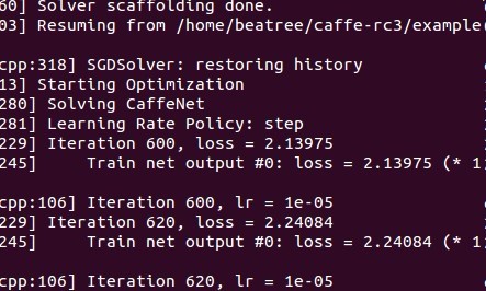
如果我们在训练途中就停电或者有了其他的情况,我们可以通过之前保存的状态恢复数据,使用的时候直接添加–snapshot参数即可,如:
.
/build/tools/caffe
train
--
solver=models/bvlc_reference_caffenet/solver
.
prototxt
--
snapshot=models/bvlc_reference_caffenet/caffenet_train_iter_10000
.
solverstate
- 1
这时候运行会从snapshot开始继续运行,如从第600迭代时运行:
1.5.5 c++ 提取特征
when everything necessary is in place:
./build/tools/extract_features
.bin
models/bvlc_reference_caffenet/bvlc_reference_caffenet
.caffemodel
examples/_temp/imagenet_val
.prototxt
fc7 examples/_temp/features
10
leveldb
- 1
the features are stored to LevelDB examples/_temp/features.
1.5.6 使用c++分类
对于c++的学习应该读读tools/caffe.cpp里的代码。
其分类命令如下:
./build/examples/cpp_classification/classification
.bin
\ models/bvlc_reference_caffenet/deploy
.prototxt
\ models/bvlc_reference_caffenet/bvlc_reference_caffenet
.caffemodel
\ data/ilsvrc12/imagenet_mean
.binaryproto
\ data/ilsvrc12/synset_words
.txt
\ examples/images/cat
.jpg
- 1
2 使用pycaffe分类
2.1 import
首先载入环境:
#
set
up Python environment: numpy
for
numerical routines,
and
matplotlib
for
plottingimport numpy
as
npimport matplotlib.pyplot
as
plt# display plots
in
this notebook%matplotlib inline#这里由于ipython启动时移除了 pylab 启动参数,所以需要使用这种格式查看,官网介绍http://ipython.org/ipython-doc/stable/interactive/reference.html#plotting-
with
-matplotlib:#
To
start
IPython
with
matplotlib support, use the --matplotlib switch.
If
IPython
is
already running, you can run the %matplotlib magic.
If
no
arguments
are
given, IPython will automatically detect your choice
of
matplotlib backend. You can also request a specific backend
with
%matplotlib backend,
where
backend must be one
of
: ‘tk’, ‘qt’, ‘wx’, ‘gtk’, ‘osx’.
In
the web notebook
and
Qt console, ‘inline’
is
also a valid backend
value
, which produces static figures inlined inside the application window instead
of
matplotlib’s interactive figures that live
in
separate windows.#
set
display defaults#关于rcParams函数http://matplotlib.org/api/matplotlib_configuration_api.html#matplotlib.rcParamsplt.rcParams[
'figure.figsize'
] = (
10
,
10
) # large imagesplt.rcParams[
'image.interpolation'
] =
'nearest'
# don
't interpolate: show square pixelsplt.rcParams['
image.cmap
'] = '
gray
' # use grayscale output rather than a (potentially misleading) color heatmap
- 1
- 2
- 3
- 4
- 5
- 6
- 7
- 8
- 9
- 10
- 11
- 12
- 13
- 14
- 15
然后
import
caffe#如果没有设置好路径可能发现不了caffe,需要
import
sys cafe_root=
'你的路径'
,sys.path.insert(
0
,caffe_root+
'python'
)之后再
import
caffe
- 1
下面下载模型,由于上面刚开始我们用的数据不是imagenet,现在我们直接下载一个模型,可能你的python中没有yaml,这里可以用pip安装(终端里):
sudo
apt-get install python-pippip install pyyaml
cd
#你的caffe root
./scripts/download_model_binary.py /home/beatree/caffe-rc3/model/bvlc_reference_caffenet
#其他的网络路径如下:models/bvlc_alexnet models/bvlc_reference_rcnn_ilsvrc13 models/bvlc_googlenet model zoo的连接http://caffe.berkeleyvision.org/model_zoo.html,模型一共232m
- 1
- 2
- 3
- 4
- 5
- 6
2.2 模型载入
caffe.set_mode_cpu()
#使用cpu模式
model_def
='/home/beatree/caffe-rc3/models/bvlc_reference_caffenet/deploy.prototxt'
model_weights
='/home/beatree/caffe-rc3/models/bvlc_reference_caffenet/bvlc_reference_caffenet.caffemodel'
net
=caffe.Net(model_def, model_weights, caffe.TEST)
mu
=np.load('/home/beatree/caffe-rc3/python/caffe/imagenet/ilsvrc_2012_mean.npy')
mu
=mu.mean(1).mean(1)
- 1
- 2
- 3
- 4
- 5
- 6
- 7
- 8
- 9
mu长成下面这个样子:
array([[[
110.17708588
,
110.45915222
,
110.68373108
,
...
,
110.9342804
,
110.79355621
,
110.5134201
], [
110.42878723
,
110.98564148
,
111.27901459
,
...
,
111.55055237
,
111.30683136
,
110.6951828
], [
110.525177
,
111.19493103
,
111.54753113
,
...
,
111.81067657
,
111.47111511
,
110.76550293
], ……
- 1
- 2
- 3
- 4
- 5
- 6
- 7
得到bgr的均值
print
'mean-subtracted values:'
, zip(
'BGR'
, mu)mean-subtracted
values
: [(
'B'
,
104.0069879317889
), (
'G'
,
116.66876761696767
), (
'R'
,
122.6789143406786
)]
- 1
- 2
- 3
- 4
matplotlib加载的image是像素[0-1],图片的数据格式[weight,high,channels],RGB 而caffe加载的图片需要的是[0-255]像素,数据格式[channels,weight,high],BGR,那么就需要转换 ,这里用了 caffe.io.Transformer,可以使用help()来获得相关信息,他的功能有
preprocess(self, in_, data)
set_channel_swap(self, in_, order)
set_input_scale(self, in_, scale)
set_mean(self, in_, mean)
set_raw_scale(self, in_, scale)
set_transpose(self, in_, order)
#
create
transformer
for
the
input
called
'data'
transformer = caffe.io.Transformer({
'data'
: net.blobs[
'data'
].data.shape})#net.blobs[
'data'
].data.shape=(
10
,
3
,
227
,
227
)transformer.set_transpose(
'data'
, (
2
,
0
,
1
)) # move image channels
to
outermost dimension第一个变成了channelstransformer.set_mean(
'data'
, mu) # subtract the dataset-mean
value
in
each
channeltransformer.set_raw_scale(
'data'
,
255
) # rescale
from
[
0
,
1
]
to
[
0
,
255
]transformer.set_channel_swap(
'data'
, (
2
,
1
,
0
)) # swap channels
from
RGB
to
BGR
- 1
- 2
- 3
- 4
- 5
- 6
- 7
- 8
2.3 cpu 分类
这里可以准备开始分类了,下面改变输入size的步骤也可以跳过,这里batchsize设置为50只是为了演示用,实际我们只对一张图片进行分类。
# set the size
of
the input (we can skip this
if
we
're
happy#
with
the
default
; we can also change it later, e.g.,
for
different batch sizes)net.blobs[
'data
'].reshape(
50
, # batch size
3
, #
3
-channel (BGR) images
227
,
227
) # image size
is
227
x227
- 1
- 2
- 3
- 4
- 5
image
= caffe.io.load_image(
'path/to/images/cat.jpg'
)transformed_image = transformer.preprocess(
'data'
,
image
)plt.imshow(
image
)
- 1
- 2
- 3
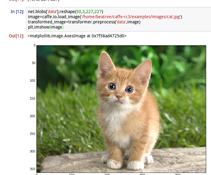
得到一个可爱的小猫,接下来看一看模型是不是认为她是不是小猫
# copy the image data into the memory allocated for the net
net.blobs[
'data'
].data[
...
] = transformed_image
### perform classification
output = net.forward()output_prob = output[
'prob'
][
0
]
# the output probability vector for the first image in the batch
print
'predicted class is:'
, output_prob.argmax(),output_prob[output_prob.argmax()]
- 1
- 2
- 3
- 4
- 5
- 6
- 7
- 8
- 9
得到结果:
predicted calss
is
281
0.312436
- 1
也就是第281种最有可能,概率比重是0.312436
那么第231种是不是猫呢,让我们接着看
# load ImageNet labels
labels_file = caffe_root +
'data/ilsvrc12/synset_words.txt'
#如果没有这个文件,须运行/data/ilsvrc12/get_ilsvrc_aux.sh
labels = np.loadtxt(labels_file, str, delimiter=
'\t'
)
print
'output label:'
, labels[output_prob.argmax()]
- 1
- 2
- 3
- 4
- 5
- 6
结果是
answer is n02123045 tabby, tabby cat
连花纹都判断对了。接下来让我们进一步观察判断的结果:
# sort top five predictions from softmax output
top
_inds = output_
prob.argsort()[
::-1
][
:5
] # reverse sort and take five largest itemsprint 'probabilities and labels:'zip(output
_prob[top_
inds], labels[top_inds])
- 1
- 2
- 3
- 4
- 5
得到的结果是:
[(
0.31243584
,
'n02123045 tabby, tabby cat'
),
#虎斑猫
(
0.2379715
,
'n02123159 tiger cat'
),
#虎猫
(
0.12387265
,
'n02124075 Egyptian cat'
),
#埃及猫
(
0.10075713
,
'n02119022 red fox, Vulpes vulpes'
),
#赤狐
(
0.070957303
,
'n02127052 lynx, catamount'
)]
#猞猁,山猫
- 1
- 2
- 3
- 4
- 5
2.4 对比GPU
现在对比下GPU与CPU的性能表现
首先看看cpu每次(50 batch size)向前运行的时间:
%
timeit
net.forward()
- 1
%timeit能自动选择运行的次数 求平均运行时间,这里我的运行时间是1 loops, best of 3: 5.29 s per loop,官网的是1.42,差距
接下来看GPU的运行时间:
caffe
.set
_device(
0
)caffe
.set
_mode_gpu()net
.forward
()%timeit net
.forward
()
- 1
- 2
- 3
- 4
1 loops, best of 3: 507 ms per loop(官网是70.2ms),慢了好多的说
2.5 查看中间输出
首先我们看下网络的结构及每层输出的shape,其形式应该是(batchsize,channeldim,height,weight)
# for each layer, show the output shape
for layer_name, blob
in
net
.blobs.iteritems
(): print layer_name +
'\t'
+ str(blob
.data.shape
)
- 1
- 2
- 3
得到的结果如下:
data
(
50
,
3
,
227
,
227
)
conv1
(
50
,
96
,
55
,
55
)
pool1
(
50
,
96
,
27
,
27
)
norm1
(
50
,
96
,
27
,
27
)
conv2
(
50
,
256
,
27
,
27
)
pool2
(
50
,
256
,
13
,
13
)
norm2
(
50
,
256
,
13
,
13
)
conv3
(
50
,
384
,
13
,
13
)
conv4
(
50
,
384
,
13
,
13
)
conv5
(
50
,
256
,
13
,
13
)
pool5
(
50
,
256
,
6
,
6
)
fc6
(
50
,
4096
)
fc7
(
50
,
4096
)
fc8
(
50
,
1000
)
prob
(
50
,
1000
)
- 1
- 2
- 3
- 4
- 5
- 6
- 7
- 8
- 9
- 10
- 11
- 12
- 13
- 14
- 15
现在看其参数的样子,函数为net.params,其中weight的样子应该是(output_channels,input_channels,filter_height,flier_width), biases的形状只有一维(output_channels,)
for layer_name,parame
in
net
.params.iteritems
():print layer_name+
'\t'
+str(param[
0
]
.shape
),str(param[
1
]
.data.shape
)
#可以看出param里0为weight1为biase
- 1
- 2
得到:
conv1 (
96
,
3
,
11
,
11
) (
96
,)
#输入3通道,输出96通道
conv2 (
256
,
48
,
5
,
5
) (
256
,)
#为什么变成48了?看下方解释
conv3 (
384
,
256
,
3
,
3
) (
384
,)
#这里的输入没变
conv4 (
384
,
192
,
3
,
3
) (
384
,)conv5 (
256
,
192
,
3
,
3
) (
256
,)fc6 (
4096
,
9216
) (
4096
,)
#9216=25*3*3
fc7 (
4096
,
4096
) (
4096
,)fc8 (
1000
,
4096
) (
1000
,)
- 1
- 2
- 3
- 4
- 5
- 6
- 7
- 8
可以看出只有卷基层和全连接层有参数
既然后了各个参数我们就初步解读下caffenet:
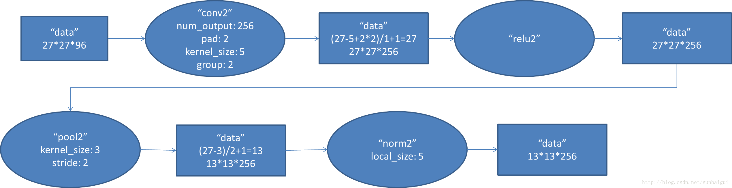
首先第一层conv1其输出结果的变化
,
这一步应该可以理解,其权重的形式为(96, 3, 11, 11)
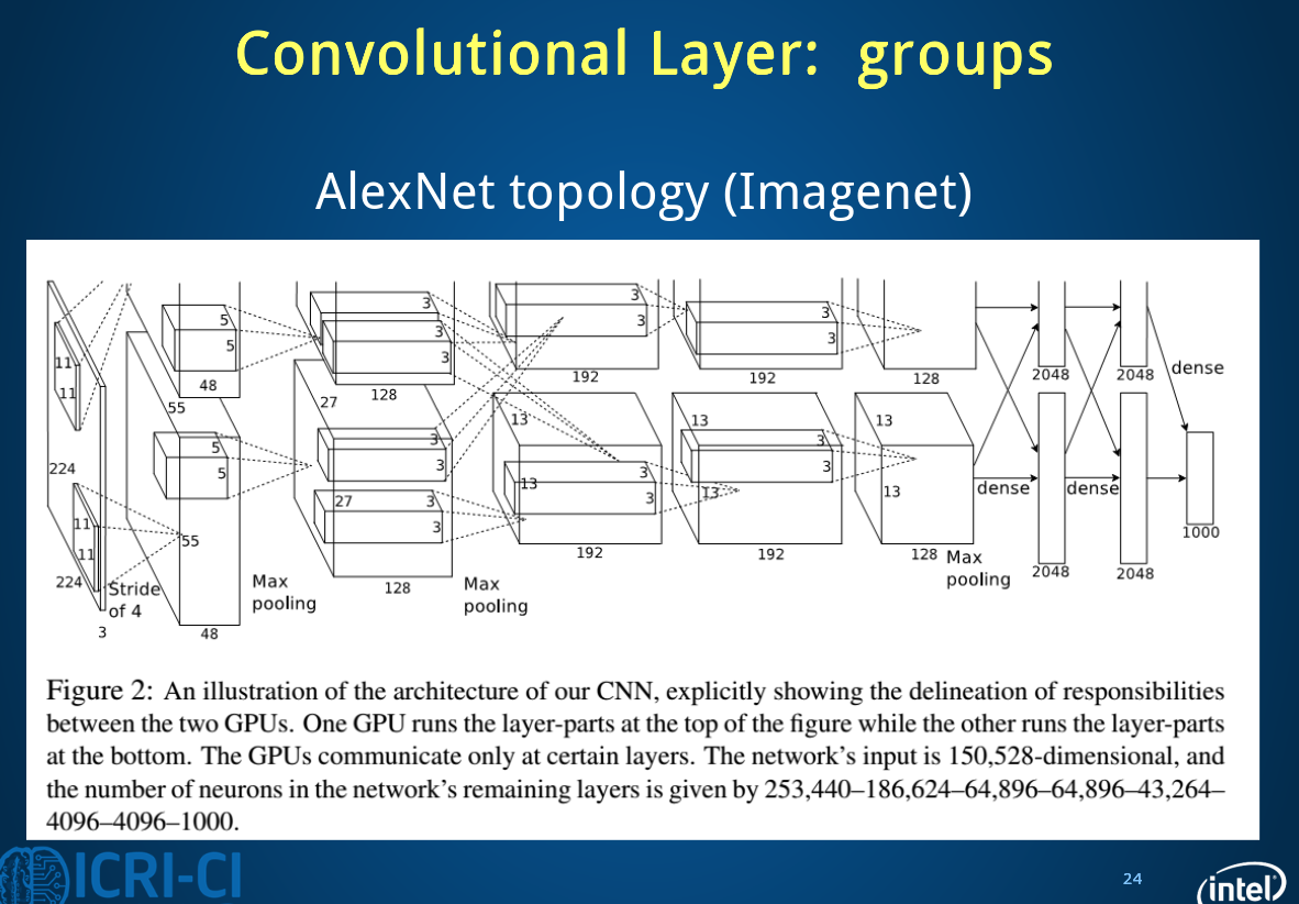
但是第二层的卷积层为什么为(256, 48, 5, 5),因为这里多了一个group选项,在cs231n里没有提及,这里的group=2,把输入输出分为了两个组也就是输入变成了96/2=48,
全连接层fc6的数据流图:
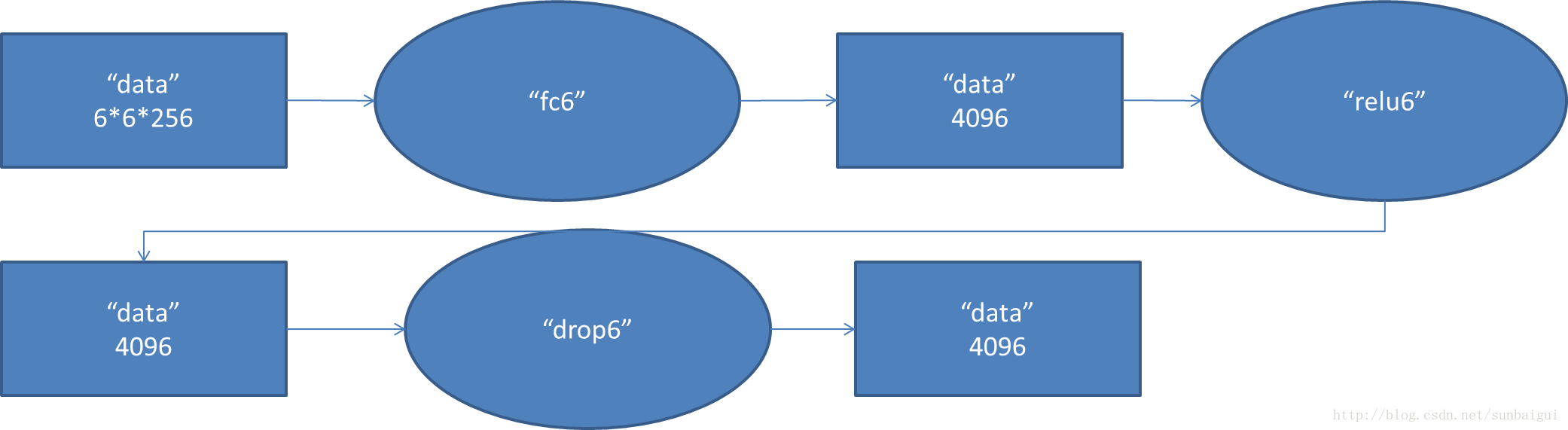
这是一张特拉维夫大学的ppt
下面进行可视化操作,首先要定义一个函数方便以后调用,可视化各层参数和结果:
def
vis_square
(data)
:
"""Take an array of shape (n, height, width) or (n, height, width, 3) and visualize each (height, width) thing in a grid of size approx. sqrt(n) by sqrt(n)"""
#输入为格式为数量,高,宽,(3),最终展示是在一个方形上
# normalize data for display
#首先将数据规则化
data = (data - data.min()) / (data.max() - data.min())
# force the number of filters to be square
n = int(np.ceil(np.sqrt(data.shape[
0
])))
#pad是补充的函数,paddign是每个纬度扩充的数量
padding = (((
0
, n **
2
- data.shape[
0
]), (
0
,
1
), (
0
,
1
))
# add some space between filters,间隔的大小
+ ((
0
,
0
),) * (data.ndim -
3
))
# don't pad the last dimension (if there is one)如果有3通道,要保持其不变
data = np.pad(data, padding, mode=
'constant'
, constant_values=
0
)
# pad with zero (black)这里该为了黑色,可以更容易看出最后一列中拓展的样子
# tile the filters into an image
data = data.reshape((n, n) + data.shape[
1
:]).transpose((
0
,
2
,
1
,
3
) + tuple(range(
4
, data.ndim +
1
))) data = data.reshape((n * data.shape[
1
], n * data.shape[
3
]) + data.shape[
4
:]) plt.imshow(data) plt.axis(
'off'
)
- 1
- 2
- 3
- 4
- 5
- 6
- 7
- 8
- 9
- 10
- 11
- 12
- 13
- 14
- 15
- 16
- 17
- 18
- 19
- 20
- 21
以conv1为例,探究如果reshape的
filters = net.params[
'conv1'
][
0
].datavis_square(filters.transpose(0, 2, 3, 1))
- 1
- 2
得到的结果
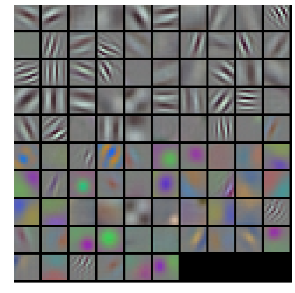
这里conv1的权重,原来的shape是(96, 3, 11, 11),其中输出为96层,每个filter的大小是11 11 3(注意后面的3噢),每个filter经过滑动窗口(卷积)得到一张output,一共得到96个。(下图是错误的,请去官网看正确的)
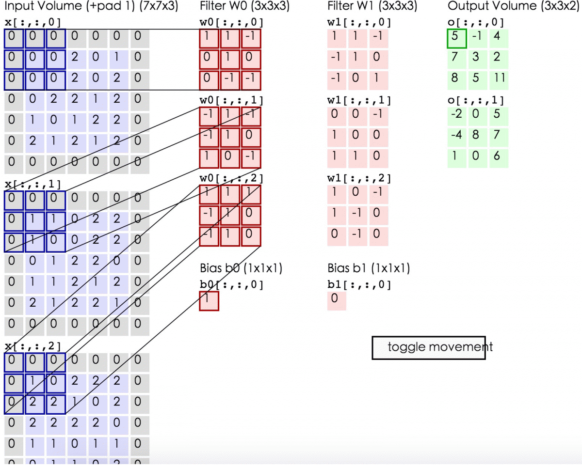
首先进入vissquare之前要transpose–》(96,11,11,3)
输入vis_square得到的padding是(0,4),(0,1),(0,1),(0,0) 也就是经过padding之后变为(100,12,12,3),这时的12多出了一个边框,第一个reshape(10,10,12,12,3),相当于原来100个图片一排变为矩阵式排列,然后又经过transpose(0,2,1,3,4)—>(10,12,10,12,3)又经过第二个reshape(120,120,3)
下面展示第一层filter输出的特征:
feat = net.blobs[
'conv1'
].data[
0
, :
36
]
#原输出为(50,96,55,55),这里取第一幅图前36张
vis_square(feat)
- 1
- 2
?
如果取全部的96张会出现下面的情况:中间的分割线没有了,为什么呢?
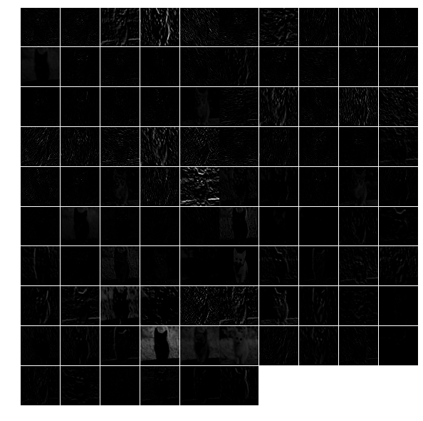
用上面的方法也可以查看其他几层的输出。
对于全连接层的输出需要用直方图的形式:
feat = net.blobs['fc6'].data[
0
]plt.subplot(
2
,
1
,
1
)plt.plot(feat.
flat
)plt.subplot(
2
,
1
,
2
)_ = plt.hist(feat.
flat
[feat.
flat
>
0
], bins=
100
)
#bin统计某一个数段之间的数量
- 1
- 2
- 3
- 4
- 5
输出分类结果:
feat
= net.blobs['prob'].
data
[0]
plt
.figure(figsize=(
15
,
3
))
plt
.plot(feat.flat)
- 1
- 2
- 3
大体就是这样了,我们可以用自己的图片来分类看看结果
2.6 总结
主要分类过程代码主要步骤:
1. 载入工具包
2. 设置显示设置
3. 设置求解其set_mode_cup()/gpu()
4. 载入模型 net=caffe.Net(,,caffe.TEST)
5. transformer(包括载入均值)
6. 设置分类输入size(batch size等)
7. 载入图片并转换(io.load_image(‘path’), transformer.preprocesss)
8. net.blobs[‘data’],data[…]=transformed_image
9. 向前计算output=net.forward
10. output_prob=output[‘prob’][0]
11. 载入synset_words.txt(np.loadtxt(,,))
12. 分类结果输出 output_prob.argsort()[::-1][]
⋆⋆⋆⋆⋆
13. 展示各层输出net.blobs.iteritems()
14. 展示各层参数net.params.iteritems()
15. 可视化注意pad和reshape,transpose的运用
16. net.params[‘name’][0].data
17. net.blobs[‘name’].data[0,:36]
18. net.blobs[‘prob’].data[0]#每个图片都有不同的输出所以后面加了个【0】
3 Fine-tuning
Now we will fine-tune the model we trained above on a different dataset to predict image style. we have 80000 images to train on. There will some changes :
1. we will change the name of the last layer form fc8 to fc8_flickr in our prototxt, it will begin
training with random weights
.
2. decrease base_lr andboost the lr_mult on the newly introduced layer.
3. set stepsize to a lower value. So the learning rate to go down faster
4. So in the solver.prototxt,we can find the base_lr is 0.001 from 0.01,and the stepsize is become to 20000 from 100000.
3.1 cmdcaffe
3.1.1 download dataset & model
we will only download 2000 images
python
.
/examples/finetune_flickr_style/assemble_data
.
py
--
workers=
-
1
--
images=2000
--
seed
831486
- 1
we have already download the model in the previous step
3.1.2 fine tune
let’s see some information in the new train_val.prototxt:
1.
ImageData later
layer{name:
"data"
type:
"ImageData"
...
transform_param{
#预处理
mirror=true crop_size:
227
#切割
mean_file:
"yourpath.binaryproto"
} image_data_param{
source
:
""
batch_size: new_height: new_width: }}
- 1
- 2
- 3
- 4
- 5
- 6
- 7
- 8
- 9
- 10
- 11
- 12
- 13
在fc8_flickr层的lr_mult分别为10和20
.
/build/tools/caffe train
-solver
models/finetune_flick_style/solver
.
prototxt
-weithts
models/bvlc_reference_caffenet/bvlc_reference_caffenet
.
caffemodel
-gpu
0
- 1
- 2
3.2 pycaffe
some functions in python :
import tempfileimage=np
.around
()image=np
.require
(image,dtype=np
.uint
8)assert os
.path.exists
(weights)
#声明,如果路径不存在会报错
。。。
- 1
- 2
- 3
- 4
- 5
在这一部分,通过ipython notebook定义了完整的网络与solver,并比较了微调模型与直接训练模型的差异,代码相对来说更加具体,由于下一边博客相关叙述比较仔细,这里就不重复了,但是还是很有必要按照官网来一遍的。
3.3 主要步骤
3.3.1 下载caffenet模型,下载Flickr数据
weights=’…..caffemodel’
3.3.2 defining and runing the nets
def
caffenet
()
:
n=caffe.NetSpec() n.data=data n.conv1,n.relu1= ...
if
train: n.drop6=fc7input=L.Dropout(n.relu6,in_place=
True
)
else
: fc7input=n.relu6
if
...
else
... fc8=L.InnerProduct(fc8input,num_output=num_clsasses,param=learned_param) n.__setattr__(classifier_name,fc8)
#classifier_name='fc8_flickr'
if
not
train: n.probs=L.Softmax(fc8)
if
label
is
not
None
: n.label=label n.loss=L.SoftmaxWithLoss(fc8,n.label) n.acc=L.Accuracy(fc8,n.label)
with
tempfile.NamedTemporaryFile(delete=
False
)
as
f: f.write(str(n.to_proto()))
return
f.name
- 1
- 2
- 3
- 4
- 5
- 6
- 7
- 8
- 9
- 10
- 11
- 12
- 13
- 14
- 15
- 16
- 17
- 18
- 19
- 20
- 21
3.3.3 dummy data imagenet
L
.DummyData
(shape=dict(dim=[
1
,
3
,
227
,
227
])) imagenet_net_filename=caffenet(data,train=False) imagenet_net=caffe
.Net
(imagenet_net_filename,weights,caffe
.TEST
)
- 1
- 2
- 3
3.3.4 style_net
have the same architecture as CaffeNet,but with differences in the input and output:
def
style_net
(traih=True,Learn_all=False,subset=None)
:
if
subset
is
None
: subset =
'train'
if
train
else
'test'
source=
'path/%s.txt'
%subset trainsfor_param=dict(mirror=train,crop_size=
227
,meanfile=
'path/xx.binaryproto'
) style_data,style_label=L.ImageData(transform_param=,source=,batch_size=,new_height=,new_width=,ntop=
2
)
return
caffenet(data=style_data,label=style_label,train=train,num_classes=
20
,classifier_name=
'fc8_filcker'
,learn_all=learn_all)
- 1
- 2
- 3
- 4
- 5
- 6
- 7
3.3.5 对比untrained_style_net,imagenet_net
3.3.6 training the style classifier
from
caffe.proto
import
caffe_pb2
def
solver
()
:
s=caffe_pb2.SloverParameter() s.train_net=train_net_path
if
test_net_path
is
not
None
: ... s.xx=xxx
with
temfile.Nxx
as
f: f.write(str(s))
return
f.name
- 1
- 2
- 3
- 4
- 5
- 6
- 7
- 8
- 9
- 10
bulit/tools/caffe train
\
-solver models/path/sovler.prototxt
\
-weights /path/.caffemodel
\
gpu 0
- 1
def
run_solvers
()
:
for
it
in
range(niter):
for
name, s
in
solvers: s.step(
1
) loss[][],acc[][]=(s.net.blobs[b].data.copy()
for
b
in
blobs)
if
it % disp_interval==
0
or
it+
1
...
print
... weight_dir=tempfile.mkdtemp() weights={}
for
name,s
in
solvers: filename= weights[name]=os.path.join(weight_dir,filename) s.net.save(weights[name])
return
loss,acc,weights
- 1
- 2
- 3
- 4
- 5
- 6
- 7
- 8
- 9
- 10
- 11
- 12
- 13
- 14
3.3.7 对比预训练效果
预训练多了一步:style_solver.net.copy_from(weights)
3.3.8 end-to-end finetuning for style
learn_all=Ture
目录


 837
837

 被折叠的 条评论
为什么被折叠?
被折叠的 条评论
为什么被折叠?
 到【灌水乐园】发言


