SSD 论文笔记

最新推荐文章于 2022-07-15 11:51:41 发布

原创最新推荐文章于 2022-07-15 11:51:41 发布

· 867 阅读

4 ·

版权

文章标签：

#深度学习 #人工智能 #神经网络

论文学习专栏收录该内容

7 篇文章

订阅专栏

摘要

We present a method for detecting objects in images using a single deep neural network. Our approach, named SSD, discretizes the output space of bounding boxes into a set of default boxes over different aspect ratios and scales per feature map location.

作者提出一个叫SSD将bounding boxes 的输出空间离散化，转换成一系列default boxes，这些default boxes 在每个特征图对应的位置上，拥有不同的aspect ratios和scales。

At prediction time, the network generates scores for the presence of each object category in each default box and produces adjustments to the box to better match the object shape. Additionally, the network combines predictions from multiple feature maps with different resolutions to naturally handle objects of various sizes.

在预测阶段，网络为每个出现的对象类别的default box打分并对default box进行调整，使其可以更好的匹配的目标的形状。此外，网络从多个特征图使用不同分辨率上进行预测，这样可以处理不同目标尺度的大小。

SSD is simple relative to methods that require object proposals because it completely eliminates proposal generation and subsequent pixel or feature resampling stages and encapsulates all computation in a single network. This makes SSD easy to train and straightforward to integrate into systems that require a detection component.

对于需要object proposals的操作，SSD的方法很简单，因为它完全消除了proposal生成以及后续的像素，或者特征图重采样的阶段，并将以上功能封装在一起使用一个单独的网络计算。这可以使得SSD很容易训练，并且直接整合到一个需要目标检测组件的系统当中。

鼎鼎大名的SSD算法，相比两阶段的faster rcnn等算法，它直接在特征图上生成defualt box，并对这些box进行调整和打分。此外，从不同分辨率的特征图上（就是不同深度的卷基层）设置default box，使其可以不同尺度的大小。（后来的FPN证明，如果没有构建横向融合的特征金字塔，对小目标的检测效果并不好，原因在于更深层的特征图有目标丰富的语义信息，通过上采样和横向融合，能够与高分辨率的特征图叠加，详见FPN）

介绍

The fundamental improvement in speed comes from eliminating bounding box proposals and the subsequent pixel or feature resampling stage. We are not the first to do this (cf [4,5]), but by adding a series of improvements, we manage to increase the accuracy significantly over previous attempts. Our improvements include using a small convolutional filter to predict object categories and offsets in bounding box locations, using separate predictors (filters) for different aspect ratio detections, and applying these filters to multiple feature maps from the later stages of a network in order to perform detection at multiple scales. With these modifications—especially using multiple layers for prediction at different scales—we can achieve high-accuracy using relatively low resolution input, further increasing detection speed.

在速度上提升的主要原因在于，消除了bounding box proposals和后续像素或特征的重采样阶段。作者不是第一个做这个事的（yolo是第一个吃螃蟹的呗），通过一系列的改进我们

SSD

SSD算法的大致框架可以用原文的如下图描述
SSD
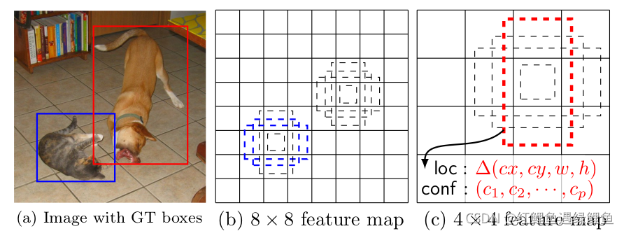
(a) SSD only needs an input image and ground truth boxes for each object during training. In a convolutional fashion, we evaluate a small set (e.g. 4) of default boxes of different aspect ratios at each location in several feature maps with different scales (e.g. 8 × 8 and 4 × 4 in (b) and ©). For each default box, we predict both the shape offsets and the confidences for all object categories ((c 1 , c 2 , · · · , c p )). At training time, we first match these default boxes to the ground truth boxes. For example, we have matched two default boxes with the cat and one with the dog, which are treated as positives and the rest as negatives. The model loss is a weighted sum between localization loss (e.g. Smooth L1 [6]) and confidence loss (e.g. Softmax).

在训练阶段，需要对应的输入图片和groud truth boxes。
首先在部分特征图上的每个位置设置一群不同aspect ratio的default boxes，如图(b)所示。对每个default box，作者预测box的shape offset和目标类别的confidences。
在训练阶段，先对default box对ground truth进行匹配。例如，现在匹配到两个default boxes，一个是猫一个是狗，这两个框按照正例（positives）处理，其余的按照负例（negatives）处理。
模型的损失函数由localization loss和confidence loss组成。

流程

借用一张网上的图片
https://blog.youkuaiyun.com/ytusdc/article/details/86577939
并参考知乎上大佬的文章
https://zhuanlan.zhihu.com/p/33544892
ssd_pipe

多尺度特征图用于检测

CNN网络特征图的分辨率随着层数加深，分辨率会逐渐减小（这种说法来自于FPN）。
在SSD中，较大分辨率的特征图和较小分辨率的特征图都会使用，大的特征图用来检测较小的目标，小的特征图用来检测较大的目标。
小的特征图使用设置的先验框尺寸较大，大的特征图设置的先验框尺寸较小。如下图，8×8的特征图和4×4的特征图，8×8的特征图设置了小的先验框，用来检测较小一点的目标。
pri_box

使用卷积进行检测

与yolo不用，SSD直接使用卷积对不同的特征图提取检测结果，如形状m×n×p的特征图，使用3×3×p的小卷积核。

设置先验框 (default box)

SSD在特征图的上的每个点，设置一系列先验框，特征图上的每个点都有数个的长宽比不同的先验框，这样每个框所对应的单元格是固定的，用于预测便捷框(bounding box)。

对于每个特征图上的每个先验框，都输出一套独立的检测值，对应一个边界框，包括两个部分内容。
第一个部分是该框对应目标的置信度（confidence），如果检测目标有c个类别，那么SSD需要预测c+1个类别的置信度，因为包括一个背景。置信度最高的类别，就是预测到的类别。

第二部分为每个先验框需要挪动的偏移量(offset)，包含四个值。
假设边界框的中心位置和高宽分别是(cx, cy, w, h)，先验框的位置用 $d=(d^{cx}, d^{cy}, d^{w}, d^{h})$ 表示，对应的边界框用
$b=(b^{cx}, b^{cy}, b^{w}, b^{h})$ ，那么预测的offset值就是下面的l
$l^{cx} = (b^{cx}-d^{cx}) / d^{w}$
$l^{cy} = (b^{cy}-d^{cy}) / d^{h}$
$l^{w} = log(b^w/d^w)$
$l^{h} = log(b^h/d^h)$

上面的过程成为边界框的编码，预测的时候需要解码，即根据先验框加上偏移量得到真实位置
$b^{cx} = d^wl^{cx} + d^{cx}$
$b^{cy} = d^yl^{cy} + d^{cy}$
$b^w = d^wexp(l^w)$
$b^h = d^hexp(l^h)$

知乎上的大佬说，在SSD的caffe源码里面还有trick，需要设置一个方差(variance)的超参数调整检测值，通过varicance_encoded_in_target来控制，如果选择该模式，需要手动设置四个方差值，边界框的解码会变成如下：

$b^{cx} = d^w * var[0] * l^{cx} + d^{cx}$
$b^{cy} = d^y * var[1] * l^{cy} + d^{cy}$
$b^w = d^wexp(var[2] * l^w)$
$b^h = d^hexp(var[3] * l^h)$

综上，对于一个m×n的特征图，每个特征图的单元设置先验框数记为k，那么每个特征图中的单元共需要(c+4)k个预测值，所有的单元共需要（c+4）kmn个预测值，因为SSD采用卷积做检测操作，所以需要(c+4)k个卷积核就可以完成这个检测过程。

backbone

SSD论文里面使用VGG16作为backbone，论文下面还有一行小字。
We use the VGG-16 network as a base, but other networks should also produce good results.
大致含义是我不想比state-of-art超过太多，所以就用来最普通的VGG16

不过作者把VGG16改了一通，全连接fc6和fc7换成了3×3卷积conv6和1×1卷积conv7，后面又添加了一系列卷积层，池化层的pool5由原来的池化核 (2,2)stride = 2换成了(3,3)stride = 1，知乎上大佬猜测是不想特征图的分辨率被弄的特别小。
此外，还用了一个膨胀卷积，扩大感受野。

作者将VGG16中的conv4_3层作为用于检测的第一个特征图，该层大小是38×38，该层非常靠前，所以norm较大，所以在后面加了一个L2 normalization，保证后面的检测层差异不大，该方法仅仅对每个像素点在channel维度上做归一化，而batch norm是在[batch, w, h]三个维度上归一化。

这个lr norm是作者后面在数据数据集进行测试的时候提了一嘴，知乎上大佬毫厘不差的总结到文章上，可见其用心。

为什么该层靠前，所以norm大？作者引用了一个parsenet网络，给出了这样的一个解释，因为conv4比较靠前（相比其他设置先验框的特征图），因此其激活之与其他层的分布较大，所以使用L2对其进行归一化操作

后面新增的卷基层中提取conv7, conv8, conv9, conv10, conv11 作为检测目标用到的特征图，加上conv4，一共6个。
特征图大小为：
(38, 38), (19, 19), (10, 10), (5, 5), (3, 3), (1, 1)
不同的特征图设置的先验框数目不同（通一个特征图上每个单元设置的先验框的数目是相同的，这里指一个单元的先验框数目）

先验框的设置包括大小和长宽比，对于大小，在每个特征图上遵循一个现行增长规则，特征图越小，先验框越大。
公式如下：
$s_k = s_{min} + \frac{s_{max}-s_{min}}{m-1}(k-1),k∈[1,m]$
上面m指特征图个数，这个值不算conv4，所以m=5，sk表示先验框大小相对于图片的比例，Smin和Smax表示比例的最大和最小值，论文里设置的是0.2和0.9。
第一个特征图先验框设置的大小比例为0.2/2 = 0.1，那么先验框尺度为300 × 0.1 = 30 （原始图像大小是300）。

后面的先验框也按照上面的公式增加，但是计算方式是先取整数再换算成比例。
ps:这里看好多博客和文献都直接把图和表贴上，而且按照公式理算出来的值还不一样，这里详细按照公式写一下计算方式。

先按照上面的公式计算得到：
s1 = 0.2, s2 = 0.375, s3 = 0.55, s4 = 0.725, s5 = 0.9
将上面的值全部扩大100倍再下取整，得到
20, 37, 55, 72, 90 (不知道知乎大佬的那个17怎么来的）
再除以100乘以图像大小，得到
sk = [30, 60, 111, 165, 216, 270]

反正我算出来是这个值，如果有知道知乎上的数值是怎么算出来，求教教我。 =_=

设置长宽比 $a_r$ 这里是aspect ratio的缩写，为[1, 2, 3, 1/2, 1/3]
先验框的长宽使用如下公式计算
$w^a_k = s_k\sqrt{a_r}, h_k^a = s_k/\sqrt{a_r}$

文中提到，每个特征图除了设置一个 $a_r = 1$ 且尺度为 $s_k$ 的先验框，还有一个 $s_k'=\sqrt{{s_k}s_{k+1}}$ 且 $a_r=1$ 的先验框，这样每个特征图就有两个长宽比为1，但是大小不同的正方形框。
因此，每个特征图的每个单元一共有{1, 2, 3, 1/2, 1/3, 1’}这么6个框，但是在实现时，conv4, conv10, conv11 仅使用4个先验框,即只保留{1, 2, 1/2, 1’}。

每个单元的先验框的中心单分布在各个单元的中心，即
$(\frac{i+0.5}{|f_k}, \frac{j+0.5}{|f_k|})，i,j∈[0,|f_k|]$
$f_k|$ 为特征图大小。

最后如整个流程的那张大图所示，SSD300会生成8732个边界框，数量很多。

训练过程

先验框匹配

训练过程要将得到的先验框与ground truth匹配，匹配上的框进行预测。
SSD中，ground truth 找到IOU最大的先验框进行匹配，并将该先验框标记为正样本。如果先验框没和任意一个ground truth匹配，那么额就和背景匹配，记为负样本。

但是在一个图片上ground truth很少，先验框很多，这样会导致负样本数量远大于正样本。所以，在上一步的基础上，如果某个未匹配的先验框与ground truth的iou大于某个阈值，那么该先验框也与ground truth匹配。
即，一个ground truth可以匹配多个多个先验框，但是一个先验框只能匹配一个ground truth。

为了保证正例与负例的样本平衡，SSD使用了hard negative mining，即对负样本排序抽样，预测为背景的置信度越小，误差越大，按照一个误差从大小排列，选取误差较大的top-k作为负样本。

这样排序的原因可以更好的区分开正样本和负样本，把模棱两可的框直接塞到负样本去。

损失函数

损失函数包括两个部分，分别是位置误差（localization loss）
和置信误差（confidence loss）的加权和

$\frac{1}{N}(Loss_{conf}(x, c) + αLoss_{loc}(x, l, g))$

N表示先验框中正样本数; $x^p_{i,j}∈{1,0}表示一个指标函数$
当 $x^p_{i,j} = 1$ 时表示第i个先验框与第j个ground truth匹配，并且类别为p。
c为类别置信度预测值，l为先验框对应边界的预测值，g为ground truth的位置参数。

计算位置误差使用 smooth L1 loss
公式敲不动了=_=

loss1 smooth 如果在训练阶段使用了variance_encoded_in_target
那么在计算loss时也要加上

在这里插入图片描述计算置信度的误差使用softmax

代码

代码参考
https://blog.youkuaiyun.com/qq_37541097/article/details/103482003

上面代码使用SSD的backbone时resnet50，不过有所改动。
原始的reset50如下图
在这里插入图片描述

仅使用了原始resnet50中conv_1到conv4_x

将conv4_block中将conv2和shortcut的conv的stride改成1

class Backbone(nn.Module):
    def __init__(self, pretrain_path=None):
        super(Backbone, self).__init__()
        net = resnet50()
        self.out_channels = [1024, 512, 512, 256, 256, 256]

        if pretrain_path is not None:
            net.load_state_dict(torch.load(pretrain_path))

        self.feature_extractor = nn.Sequential(*list(net.children())[:7]) # net.children是网络中的self成员，取前7个

        conv4_block1 = self.feature_extractor[-1][0] # 取出conv4_block 的第一个bottlenect(带一个downsample) 

        # 修改conv4_block1的步距，从2->1
        conv4_block1.conv1.stride = (1, 1) # 这个本来stride就是1 =_=
        conv4_block1.conv2.stride = (1, 1)
        conv4_block1.downsample[0].stride = (1, 1)

    def forward(self, x):
        x = self.feature_extractor(x)
        return x

输出原始的conv4_block1图结构如下

Bottleneck(
  (conv1): Conv2d(512, 256, kernel_size=(1, 1), stride=(1, 1), bias=False)
  (bn1): BatchNorm2d(256, eps=1e-05, momentum=0.1, affine=True, track_running_stats=True)
  (conv2): Conv2d(256, 256, kernel_size=(3, 3), stride=(2, 2), padding=(1, 1), bias=False) #这个stride改成1
  (bn2): BatchNorm2d(256, eps=1e-05, momentum=0.1, affine=True, track_running_stats=True)
  (conv3): Conv2d(256, 1024, kernel_size=(1, 1), stride=(1, 1), bias=False)
  (bn3): BatchNorm2d(1024, eps=1e-05, momentum=0.1, affine=True, track_running_stats=True)
  (relu): ReLU(inplace=True)
  (downsample): Sequential(
    (0): Conv2d(512, 1024, kernel_size=(1, 1), stride=(2, 2), bias=False)# 这个stride改成1
    (1): BatchNorm2d(1024, eps=1e-05, momentum=0.1, affine=True, track_running_stats=True)
  )
)

后面接上作者自己定义的additional_features，用来提取特征图中的location和score等信息

下面代码时SSD300的定义，先看__init__部分

class SSD300(nn.Module):
    def __init__(self, backbone=None, num_classes=21):
        super(SSD300, self).__init__()
        if backbone is None:
            raise Exception("backbone is None")
        if not hasattr(backbone, "out_channels"):
            raise Exception("the backbone not has attribute: out_channel")
        self.feature_extractor = backbone

        self.num_classes = num_classes
        # out_channels = [1024, 512, 512, 256, 256, 256] for resnet50
        self._build_additional_features(self.feature_extractor.out_channels) # conv4后面接的额外添加的卷积层
        self.num_defaults = [4, 6, 6, 6, 4, 4] # 每个层feature map上每个点生成的default box数量
        location_extractors = []
        confidence_extractors = []

        # out_channels = [1024, 512, 512, 256, 256, 256] for resnet50
        for nd, oc in zip(self.num_defaults, self.feature_extractor.out_channels):
            # nd is number_default_boxes, oc is output_channel
            location_extractors.append(nn.Conv2d(oc, nd * 4, kernel_size=3, padding=1)) # nd * 4表示nd个default box对应的4个坐标
            confidence_extractors.append(nn.Conv2d(oc, nd * self.num_classes, kernel_size=3, padding=1)) # nd * self.num_classes表示每个default box在每个类别上的概率

        self.loc = nn.ModuleList(location_extractors)
        self.conf = nn.ModuleList(confidence_extractors)
        self._init_weights()

        default_box = dboxes300_coco()
        self.compute_loss = Loss(default_box) #计算box的损失
        self.encoder = Encoder(default_box) #将输入的default box计算iou并修改default box的描述格式
        self.postprocess = PostProcess(default_box)# 将预测到的回归参数应用到default box上并选出最佳的预测框

    def _build_additional_features(self, input_size):
        pass
    def _init_weights(self):
        pass
    def bbox_view(self, features, loc_extractor, conf_extractor):
        pass
    def forward(self, image, targets=None):
        pass

_build_additional_features函数是作者在renset50去掉conv5_x以及后面的层后，新添加的5个层结构，每个层中包含两个conv, bn以及relu

    def _build_additional_features(self, input_size):
        """
        为backbone(resnet50)添加额外的一系列卷积层，得到相应的一系列特征提取器
        :param input_size:
        :return:
        """
        additional_blocks = []
        # input_size = [1024, 512, 512, 256, 256, 256] for resnet50
        middle_channels = [256, 256, 128, 128, 128]
        for i, (input_ch, output_ch, middle_ch) in enumerate(zip(input_size[:-1], input_size[1:], middle_channels)):
            padding, stride = (1, 2) if i < 3 else (0, 1) # 0，1，2的pad和stride分别是(1,2)
            layer = nn.Sequential(
                nn.Conv2d(input_ch, middle_ch, kernel_size=1, bias=False),
                nn.BatchNorm2d(middle_ch),
                nn.ReLU(inplace=True),
                nn.Conv2d(middle_ch, output_ch, kernel_size=3, padding=padding, stride=stride, bias=False),
                nn.BatchNorm2d(output_ch),
                nn.ReLU(inplace=True),
            )
            additional_blocks.append(layer)
        self.additional_blocks = nn.ModuleList(additional_blocks)

_init_weights 就是对网络权重执行初始化的操作

    def _init_weights(self):
        layers = [*self.additional_blocks, *self.loc, *self.conf]
        for layer in layers:
            for param in layer.parameters():
                if param.dim() > 1:
                    nn.init.xavier_uniform_(param) # 可以看到使用xavier初始化

bbox_view函数，输入三个参数，分别是特征图（包括backbone以及additional_layer），用于预测位置的卷积层结果，用于预测目标概率的卷积层结果。
该函数的功能是把输入的各种特征图信息，转换shape并对location以及confidence的特征图进行拼接

		# 
    def bbox_view(self, features, loc_extractor, conf_extractor):
        locs = []
        confs = []
        for f, l, c in zip(features, loc_extractor, conf_extractor):
            # [batch, n*4, feat_size, feat_size] -> [batch, 4, -1]
            locs.append(l(f).view(f.size(0), 4, -1))
            # [batch, n*classes, feat_size, feat_size] -> [batch, classes, -1]
            confs.append(c(f).view(f.size(0), self.num_classes, -1))
				# 注意这里的locs和confs都是list，相当于在list上做拼接
        locs, confs = torch.cat(locs, 2).contiguous(), torch.cat(confs, 2).contiguous()
        return locs, confs

最后看forward操作，主要包含三个过程：
1.提取特征图 2.计算loss（如果是训练模式) 3.得到预测结果（postprocess)

    def forward(self, image, targets=None):
        x = self.feature_extractor(image)

        # Feature Map 38x38x1024, 19x19x512, 10x10x512, 5x5x256, 3x3x256, 1x1x256
        detection_features = torch.jit.annotate(List[Tensor], [])  # [x]
        detection_features.append(x)
        for layer in self.additional_blocks:
            x = layer(x)
            detection_features.append(x)

        # Feature Map 38x38x4, 19x19x6, 10x10x6, 5x5x6, 3x3x4, 1x1x4
        locs, confs = self.bbox_view(detection_features, self.loc, self.conf)

        # For SSD 300, shall return nbatch x 8732 x {nlabels, nlocs} results
        # 38x38x4 + 19x19x6 + 10x10x6 + 5x5x6 + 3x3x4 + 1x1x4 = 8732

        if self.training:
            if targets is None:
                raise ValueError("In training mode, targets should be passed")
            # bboxes_out (Tensor 8732 x 4), labels_out (Tensor 8732)
            bboxes_out = targets['boxes']
            bboxes_out = bboxes_out.transpose(1, 2).contiguous()
            # print(bboxes_out.is_contiguous())
            labels_out = targets['labels']
            # print(labels_out.is_contiguous())

            # ploc, plabel, gloc, glabel
            loss = self.compute_loss(locs, confs, bboxes_out, labels_out)
            return {"total_losses": loss}

        # 将预测回归参数叠加到default box上得到最终预测box，并执行非极大值抑制虑除重叠框
        results = self.postprocess(locs, confs)
        return results

loss类构造函数传入的参数是每个特征图上设置的default box

def dboxes300_coco():
    figsize = 300  # 输入网络的图像大小
    feat_size = [38, 19, 10, 5, 3, 1]   # 每个预测层的feature map尺寸
    steps = [8, 16, 32, 64, 100, 300]   # 每个特征层上的一个cell在原图上的跨度
    # use the scales here: https://github.com/amdegroot/ssd.pytorch/blob/master/data/config.py
    scales = [21, 45, 99, 153, 207, 261, 315]  # 每个特征层上预测的default box的scale
    aspect_ratios = [[2], [2, 3], [2, 3], [2, 3], [2], [2]]  # 每个预测特征层上预测的default box的ratios
    dboxes = DefaultBoxes(figsize, feat_size, steps, scales, aspect_ratios) #返回default box
    return dboxes

Loss计算

class Loss(nn.Module):
    """
        Implements the loss as the sum of the followings:
        1. Confidence Loss: All labels, with hard negative mining
        2. Localization Loss: Only on positive labels
        Suppose input dboxes has the shape 8732x4
    """
    def __init__(self, dboxes):
        super(Loss, self).__init__()
        # Two factor are from following links
        # http://jany.st/post/2017-11-05-single-shot-detector-ssd-from-scratch-in-tensorflow.html
        # 超参数
        self.scale_xy = 1.0 / dboxes.scale_xy  # 10
        self.scale_wh = 1.0 / dboxes.scale_wh  # 5

        self.location_loss = nn.SmoothL1Loss(reduction='none')
        # [num_anchors, 4] -> [4, num_anchors] -> [1, 4, num_anchors]
        self.dboxes = nn.Parameter(dboxes(order="xywh").transpose(0, 1).unsqueeze(dim=0),
                                   requires_grad=False)

        self.confidence_loss = nn.CrossEntropyLoss(reduction='none')

    def _location_vec(self, loc):
        pass
    def forward(self, ploc, plabel, gloc, glabel):
        pass

_location_vec函数，将预测的位置回归信息应用到default box上

    def _location_vec(self, loc):
        # type: (Tensor) -> Tensor
        """
        Generate Location Vectors
        计算ground truth相对anchors的回归参数
        :param loc: anchor匹配到的对应GTBOX Nx4x8732
        :return:
        """
        gxy = self.scale_xy * (loc[:, :2, :] - self.dboxes[:, :2, :]) / self.dboxes[:, 2:, :]  # Nx2x8732
        gwh = self.scale_wh * (loc[:, 2:, :] / self.dboxes[:, 2:, :]).log()  # Nx2x8732
        return torch.cat((gxy, gwh), dim=1).contiguous()

loss计算的forward函数传入的参数包含四个内容，分别是预测的位置回归参数，预测的类别标签，在数据预处理时处理好的anhor匹配到的ground true以及label的真实标签，计算过程包括计算loss以及如何对negtive instance进行选取和处理

 def forward(self, ploc, plabel, gloc, glabel):
        # type: (Tensor, Tensor, Tensor, Tensor) -> Tensor
        """
            ploc, plabel: Nx4x8732, Nxlabel_numx8732
                predicted location and labels

            gloc, glabel: Nx4x8732, Nx8732
                ground truth location and labels
        """
        # 获取正样本的mask  Tensor: [N, 8732]
        mask = torch.gt(glabel, 0)  # (gt: >)
        # mask1 = torch.nonzero(glabel)
        # 计算一个batch中的每张图片的正样本个数 Tensor: [N]
        pos_num = mask.sum(dim=1)

        # 计算gt的location回归参数 Tensor: [N, 4, 8732]
        vec_gd = self._location_vec(gloc)

        # sum on four coordinates, and mask
        # 计算定位损失(只有正样本)
        loc_loss = self.location_loss(ploc, vec_gd).sum(dim=1)  # Tensor: [N, 8732]
        loc_loss = (mask.float() * loc_loss).sum(dim=1)  # Tenosr: [N] 去掉所有负样本的损失

        # hard negative mining Tenosr: [N, 8732]
        con = self.confidence_loss(plabel, glabel)

        # positive mask will never selected
        # 获取负样本
        con_neg = con.clone()
        con_neg[mask] = 0.0
        # 按照confidence_loss降序排列 con_idx(Tensor: [N, 8732])
        _, con_idx = con_neg.sort(dim=1, descending=True)
        _, con_rank = con_idx.sort(dim=1)  # 把数据先升序排列，得到下标，再对下标降序排列，找出小于2的，就是最大的两个数对应的位置
        #[0.3, 0.1, 0, 0.5, 0.2]
        #[3, 0, 4, 1, 2]
        #[1, 3, 4, 0, 2] < 2
        #[1, 0, 0, 1, 0]

        # number of negative three times positive
        # 用于损失计算的负样本数是正样本的3倍（在原论文Hard negative mining部分），
        # 但不能超过总样本数8732
        neg_num = torch.clamp(3 * pos_num, max=mask.size(1)).unsqueeze(-1)
        neg_mask = torch.lt(con_rank, neg_num)  # (lt: <) Tensor [N, 8732]

        # confidence最终loss使用选取的正样本loss+选取的负样本loss
        con_loss = (con * (mask.float() + neg_mask.float())).sum(dim=1)  # Tensor [N]

        # avoid no object detected
        # 避免出现图像中没有GTBOX的情况
        total_loss = loc_loss + con_loss
        # eg. [15, 3, 5, 0] -> [1.0, 1.0, 1.0, 0.0]
        num_mask = torch.gt(pos_num, 0).float()  # 统计一个batch中的每张图像中是否存在正样本
        pos_num = pos_num.float().clamp(min=1e-6)  # 防止出现分母为零的情况
        ret = (total_loss * num_mask / pos_num).mean(dim=0)  # 只计算存在正样本的图像损失, pos_num就是论文里面的N表示正样本的个数
        return ret

计算Loss时拿到的ground true 必须是和default box匹配上的，匹配过程中使用了另一个类，Encoder类，匹配的代码如下：

class AssignGTtoDefaultBox(object):
    def __init__(self):
        self.default_box = dboxes300_coco() # 这里拿到ssd300 default box的scale aspect_ratio等信息
        self.encoder = Encoder(self.default_box) # 调用encoder方法进行匹配

    def __call__(self, image, target):
        boxes = target['boxes']
        labels = target["labels"]
        # bboxes_out (Tensor 8732 x 4), labels_out (Tensor 8732)
        bboxes_out, labels_out = self.encoder.encode(boxes, labels)
        target['boxes'] = bboxes_out
        target['labels'] = labels_out

        return image, target

Encoder 类（部分）如下

class Encoder(object):
    """
        Inspired by https://github.com/kuangliu/pytorch-src
        Transform between (bboxes, lables) <-> SSD output

        dboxes: default boxes in size 8732 x 4,
            encoder: input ltrb format, output xywh format
            decoder: input xywh format, output ltrb format

        encode:
            input  : bboxes_in (Tensor nboxes x 4), labels_in (Tensor nboxes)
            output : bboxes_out (Tensor 8732 x 4), labels_out (Tensor 8732)
            criteria : IoU threshold of bboexes

        decode:
            input  : bboxes_in (Tensor 8732 x 4), scores_in (Tensor 8732 x nitems)
            output : bboxes_out (Tensor nboxes x 4), labels_out (Tensor nboxes)
            criteria : IoU threshold of bboexes
            max_output : maximum number of output bboxes
    """
    def __init__(self, dboxes):
        self.dboxes = dboxes(order='ltrb')
        self.dboxes_xywh = dboxes(order='xywh').unsqueeze(dim=0)
        self.nboxes = self.dboxes.size(0)  # default boxes的数量
        self.scale_xy = dboxes.scale_xy
        self.scale_wh = dboxes.scale_wh

    def encode(self, bboxes_in, labels_in, criteria=0.5):
        """
        encode:
            input  : bboxes_in (Tensor nboxes x 4), labels_in (Tensor nboxes)
            output : bboxes_out (Tensor 8732 x 4), labels_out (Tensor 8732)
            criteria : IoU threshold of bboexes
        """
        # 计算iou的函数
        ious = calc_iou_tensor(bboxes_in, self.dboxes)   # [nboxes, 8732]
        # [8732,]
        best_dbox_ious, best_dbox_idx = ious.max(dim=0)  # 寻找每个default box匹配到的最大IoU bboxes_in
        # [nboxes,]
        best_bbox_ious, best_bbox_idx = ious.max(dim=1)  # 寻找每个bboxes_in匹配到的最大IoU default box

        # set best ious 2.0
        # 将每个bboxes_in匹配到的最佳default box设置为正样本（对应论文中Matching strategy的第一条）
        best_dbox_ious.index_fill_(0, best_bbox_idx, 2.0)

        # 将相应default box的匹配最大IoU bboxes_in信息替换成best_bbox_idx
        idx = torch.arange(0, best_bbox_idx.size(0), dtype=torch.int64)
        best_dbox_idx[best_bbox_idx[idx]] = idx

        # filter IoU > 0.5
        # 寻找与bbox_in iou大于0.5的default box,对应论文中Matching strategy的第二条(这里包括了第一条匹配到的信息)
        masks = best_dbox_ious > criteria
        # [8732,]
        labels_out = torch.zeros(self.nboxes, dtype=torch.int64)
        labels_out[masks] = labels_in[best_dbox_idx[masks]]
        bboxes_out = self.dboxes.clone()
        # 将default box匹配到正样本的地方设置成对应正样本box信息
        bboxes_out[masks, :] = bboxes_in[best_dbox_idx[masks], :]
        # Transform format to xywh format
        x = 0.5 * (bboxes_out[:, 0] + bboxes_out[:, 2])  # x
        y = 0.5 * (bboxes_out[:, 1] + bboxes_out[:, 3])  # y
        w = bboxes_out[:, 2] - bboxes_out[:, 0]  # w
        h = bboxes_out[:, 3] - bboxes_out[:, 1]  # h
        bboxes_out[:, 0] = x
        bboxes_out[:, 1] = y
        bboxes_out[:, 2] = w
        bboxes_out[:, 3] = h
        return bboxes_out, labels_out

最后看后处理部分，将计算得到的位置偏移参数和目标框的概率添加到预测的box上

初始化参数传入default box，forward参数传入预测的box位置偏移以及预测的类别概率

class PostProcess(nn.Module):
    def __init__(self, dboxes):
        super(PostProcess, self).__init__()
        # [num_anchors, 4] -> [1, num_anchors, 4]
        self.dboxes_xywh = nn.Parameter(dboxes(order='xywh').unsqueeze(dim=0),
                                        requires_grad=False)
        self.scale_xy = dboxes.scale_xy  # 0.1
        self.scale_wh = dboxes.scale_wh  # 0.2
			 
			  # iou阈值
        self.criteria = 0.5
			  # 最多输出100个目标
        self.max_output = 100

    def scale_back_batch(self, bboxes_in, scores_in):
        pass

    def decode_single_new(self, bboxes_in, scores_in, criteria, num_output):
        pass

    def forward(self, bboxes_in, scores_in):
        pass

下面是后处理部分的forward函数，先将box的回归信息添加到default box上，获得所有预测的box的位置。
再通过decode_single_new函数计算nms，选出最佳的目标检测框

		# 传入的是预测的box的回归信息以及分数
    def forward(self, bboxes_in, scores_in):
        # 通过预测的boxes回归参数得到最终预测坐标, 将预测目标score通过softmax处理
        bboxes, probs = self.scale_back_batch(bboxes_in, scores_in)

        outputs = torch.jit.annotate(List[Tuple[Tensor, Tensor, Tensor]], [])
        # 遍历一个batch中的每张image数据
        # bboxes: [batch, 8732, 4]
        for bbox, prob in zip(bboxes.split(1, 0), probs.split(1, 0)):  # split_size, split_dim
            # bbox: [1, 8732, 4]
            bbox = bbox.squeeze(0)
            prob = prob.squeeze(0)
            outputs.append(self.decode_single_new(bbox, prob, self.criteria, self.max_output))
        return outputs

先看scale_back_batch 函数

    def scale_back_batch(self, bboxes_in, scores_in):
        # type: (Tensor, Tensor) -> Tuple[Tensor, Tensor]
        """
            1）通过预测的boxes回归参数得到最终预测坐标
            2）将box格式从xywh转换回ltrb
            3）将预测目标score通过softmax处理
            Do scale and transform from xywh to ltrb
            suppose input N x 4 x num_bbox | N x label_num x num_bbox

            bboxes_in: [N, 4, 8732]是网络预测的xywh回归参数
            scores_in: [N, label_num, 8732]是预测的每个default box的各目标概率
        """
        # Returns a view of the original tensor with its dimensions permuted.
        # [batch, 4, 8732] -> [batch, 8732, 4]
        bboxes_in = bboxes_in.permute(0, 2, 1)
        # [batch, label_num, 8732] -> [batch, 8732, label_num]
        scores_in = scores_in.permute(0, 2, 1)
        # print(bboxes_in.is_contiguous())

        bboxes_in[:, :, :2] = self.scale_xy * bboxes_in[:, :, :2]   # 预测的x, y回归参数
        bboxes_in[:, :, 2:] = self.scale_wh * bboxes_in[:, :, 2:]   # 预测的w, h回归参数

        # 将预测的回归参数叠加到default box上得到最终的预测边界框
        bboxes_in[:, :, :2] = bboxes_in[:, :, :2] * self.dboxes_xywh[:, :, 2:] + self.dboxes_xywh[:, :, :2]
        bboxes_in[:, :, 2:] = bboxes_in[:, :, 2:].exp() * self.dboxes_xywh[:, :, 2:]

        # transform format to ltrb
        l = bboxes_in[:, :, 0] - 0.5 * bboxes_in[:, :, 2]
        t = bboxes_in[:, :, 1] - 0.5 * bboxes_in[:, :, 3]
        r = bboxes_in[:, :, 0] + 0.5 * bboxes_in[:, :, 2]
        b = bboxes_in[:, :, 1] + 0.5 * bboxes_in[:, :, 3]

        bboxes_in[:, :, 0] = l  # xmin
        bboxes_in[:, :, 1] = t  # ymin
        bboxes_in[:, :, 2] = r  # xmax
        bboxes_in[:, :, 3] = b  # ymax

        # scores_in: [batch, 8732, label_num]
        return bboxes_in, F.softmax(scores_in, dim=-1)

最后decode_single_new函数，对所有得到的预测框进行处理，并进行nms操作得到最终结果

    def decode_single_new(self, bboxes_in, scores_in, criteria, num_output):
        # type: (Tensor, Tensor, float, int) -> Tuple[Tensor, Tensor, Tensor]
        """
        decode:
            input  : bboxes_in (Tensor 8732 x 4), scores_in (Tensor 8732 x nitems)
            output : bboxes_out (Tensor nboxes x 4), labels_out (Tensor nboxes)
            criteria : IoU threshold of bboexes
            max_output : maximum number of output bboxes
        """
        device = bboxes_in.device
        num_classes = scores_in.shape[-1]

        # 对越界的bbox进行裁剪
        bboxes_in = bboxes_in.clamp(min=0, max=1)

        # [8732, 4] -> [8732, 21, 4]
        bboxes_in = bboxes_in.repeat(1, num_classes).reshape(scores_in.shape[0], -1, 4)

        # create labels for each prediction
        labels = torch.arange(num_classes, device=device)
        # [num_classes] -> [8732, num_classes]
        labels = labels.view(1, -1).expand_as(scores_in)

        # remove prediction with the background label
        # 移除归为背景类别的概率信息
        bboxes_in = bboxes_in[:, 1:, :]  # [8732, 21, 4] -> [8732, 20, 4]
        scores_in = scores_in[:, 1:]  # [8732, 21] -> [8732, 20]
        labels = labels[:, 1:]  # [8732, 21] -> [8732, 20]

        # batch everything, by making every class prediction be a separate instance
        bboxes_in = bboxes_in.reshape(-1, 4)  # [8732, 20, 4] -> [8732x20, 4]
        scores_in = scores_in.reshape(-1)  # [8732, 20] -> [8732x20]
        labels = labels.reshape(-1)  # [8732, 20] -> [8732x20]

        # remove low scoring boxes
        # 移除低概率目标，self.scores_thresh=0.05
        # inds = torch.nonzero(scores_in > 0.05).squeeze(1)
        inds = torch.where(torch.gt(scores_in, 0.05))[0]
        bboxes_in, scores_in, labels = bboxes_in[inds, :], scores_in[inds], labels[inds]

        # remove empty boxes
        ws, hs = bboxes_in[:, 2] - bboxes_in[:, 0], bboxes_in[:, 3] - bboxes_in[:, 1]
        keep = (ws >= 1 / 300) & (hs >= 1 / 300)
        # keep = keep.nonzero().squeeze(1)
        keep = torch.where(keep)[0]
        bboxes_in, scores_in, labels = bboxes_in[keep], scores_in[keep], labels[keep]

        # non-maximum suppression
        keep = batched_nms(bboxes_in, scores_in, labels, iou_threshold=criteria)

        # keep only topk scoring predictions
        keep = keep[:num_output]
        bboxes_out = bboxes_in[keep, :]
        scores_out = scores_in[keep]
        labels_out = labels[keep]

        return bboxes_out, labels_out, scores_out