机器学习笔记 -吴恩达（第六章：线性回归，numpy实现、scikit-learn实现，附源码）

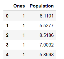
（1）数据描述

1，使用pandas读取数据，简化后续操作

import numpy as np
import pandas as pd
import matplotlib.pyplot as plt

path =  'ex1data1.txt'
data = pd.read_csv(path, header=None, names=['Population', 'Profit'])
data.head()

2，绘制数据，看看数据样子

data.plot(kind='scatter', x='Population', y='Profit', figsize=(12,8))
plt.show()

3，定义一个损失函数，使用梯度下降算法

    def computeCost(X, y, theta):
          inner = np.power(((X * theta.T) - y), 2)
          return np.sum(inner) / (2 * len(X))

    公式 ：

4，为了使用向量进行计算，对数据做一些改造

   在训练集中添加一列，以便我们可以使用向量化的解决方案来计算代价和梯度。

  data.insert(0, 'Ones', 1)

 cols = data.shape[1]

 #特征数据集
 X = data.iloc[:,0:cols-1]#X是所有行，去掉最后一列

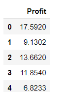
#目标数据集
 y = data.iloc[:,cols-1:cols]#X是所有行，只取最后一列

X.head()#head()是观察前5行

y.head()

5，数据预处理

代价函数是应该是numpy矩阵，所以我们需要转换X和Y， 需要初始化theta。

X = np.matrix(X.values)
print (X)
y = np.matrix(y.values)
print (y)
theta = np.matrix(np.array([0,0]))
print (theta)

6，计算损失函数 theta初始化为0时候

computeCost(X, y, theta)

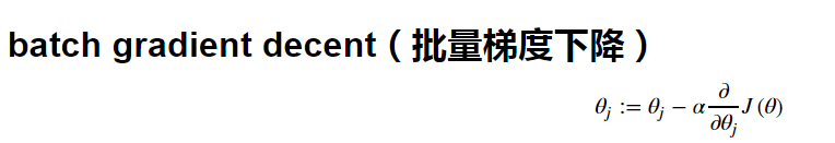
7，批量梯度下降算法定义

公式：

def gradientDescent(X, y, theta, alpha, iters):
    #[[0. 0.]]
    temp = np.matrix(np.zeros(theta.shape))
    #2
    parameters = int(theta.ravel().shape[1])
    #预定义10000个损失值，初始化为0
    cost = np.zeros(iters)
    #每循环一次，计算一次损失值，并赋值
    for i in range(iters):
        #误差矩阵
        error = (X * theta.T) - y
        print  (error)
        #更新参数值,统一全部更新
        for j in range(parameters):
            term = np.multiply(error, X[:,j])
            temp[0,j] = theta[0,j] - ((alpha / len(X)) * np.sum(term))            
        theta = temp

        # 计算损失值并保存
        cost[i] = computeCost(X, y, theta)        
    return theta, cost

 

8，设置学习率，迭代次数

alpha = 0.01
iters = 1000

9，开始使用批量梯度下降算法进行计算

g, cost = gradientDescent(X, y, theta, alpha, iters)
print (g)
print (cost)

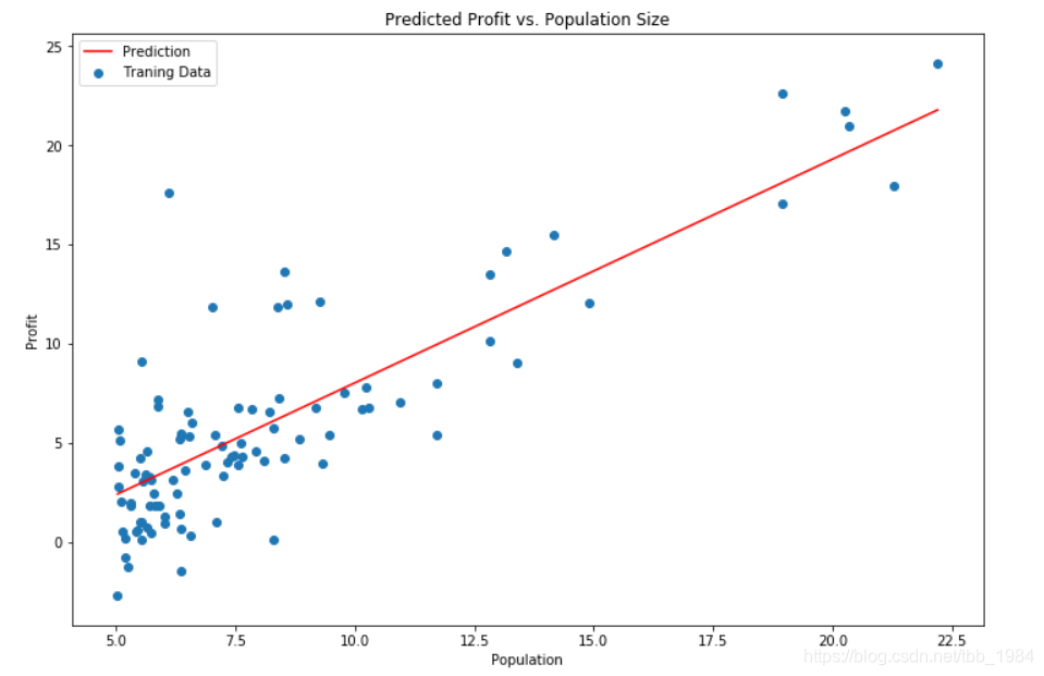
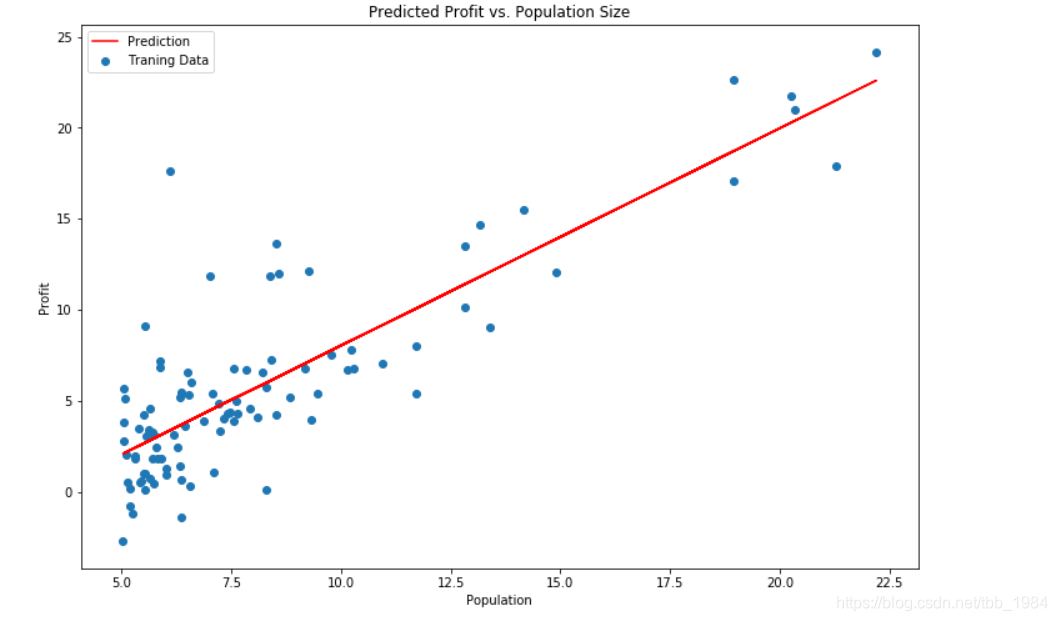
10，绘制一下拟合情况

x = np.linspace(data.Population.min(), data.Population.max(), 100)
f = g[0, 0] + (g[0, 1] * x)

fig, ax = plt.subplots(figsize=(12,8))
ax.plot(x, f, 'r', label='Prediction')
ax.scatter(data.Population, data.Profit, label='Traning Data')
ax.legend(loc=2)
ax.set_xlabel('Population')
ax.set_ylabel('Profit')
ax.set_title('Predicted Profit vs. Population Size')
plt.show()

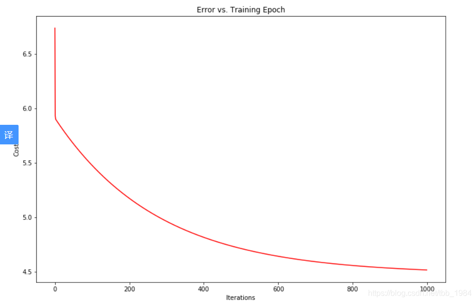
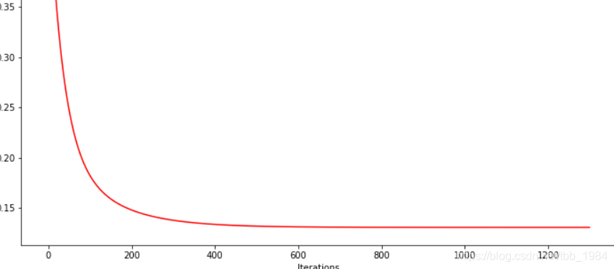
11  绘制一下训练次数与损失函数的关系

fig, ax = plt.subplots(figsize=(12,8))
ax.plot(np.arange(iters), cost, 'r')
ax.set_xlabel('Iterations')
ax.set_ylabel('Cost')
ax.set_title('Error vs. Training Epoch')
plt.show()

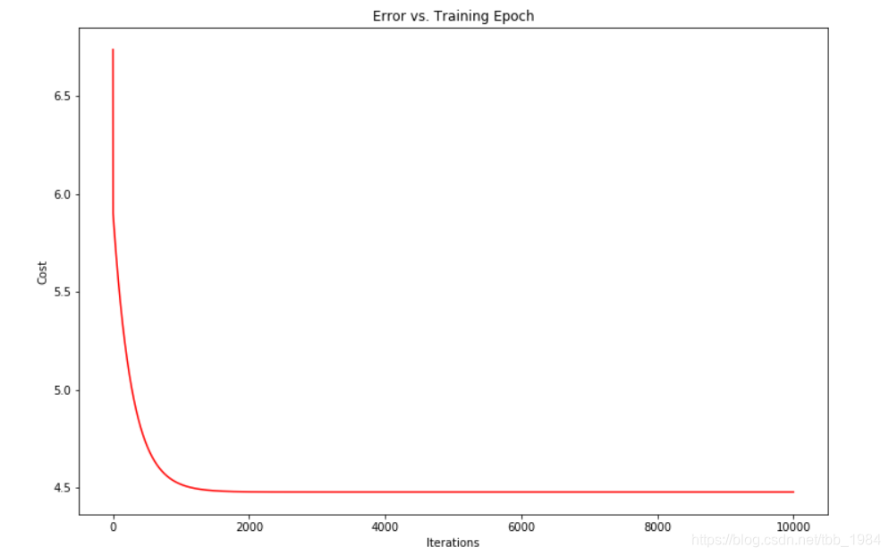
迭代次数修改为10000次，发现其实到2000次左右，损失函数基本上就不再变小了

多变量线性回归

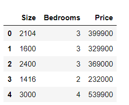
1,数据描述

房屋价格数据集，其中有2个变量（房子的大小，卧室的数量）和目标（房子的价格）。 

path =  'ex1data2.txt'
data2 = pd.read_csv(path, header=None, names=['Size', 'Bedrooms', 'Price'])
data2.head()

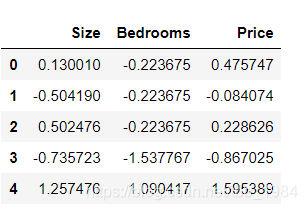
2，特征归一化处理

由于特征值大小差别太大，会影响寻找损失函数最优值的速度，我们添加了另一个预处理步骤 - 特征归一化。 这个对于pandas来说很简单

data2 = (data2 - data2.mean()) / data2.std()
data2.head()

3，数据预处理

# 添加一列
data2.insert(0, 'Ones', 1)

cols = data2.shape[1]

#特征集
X2 = data2.iloc[:,0:cols-1]

#目标集
y2 = data2.iloc[:,cols-1:cols]

# 转换为矩阵
X2 = np.matrix(X2.values)
y2 = np.matrix(y2.values)

#参数初始化
theta2 = np.matrix(np.array([0,0,0]))

# 多变量线性回归训练
g2, cost2 = gradientDescent(X2, y2, theta2, alpha, iters)

# 获取损失函数值
computeCost(X2, y2, g2)

4，查看训练过程

fig, ax = plt.subplots(figsize=(12,8))
ax.plot(np.arange(iters), cost2, 'r')
ax.set_xlabel('Iterations')
ax.set_ylabel('Cost')
ax.set_title('Error vs. Training Epoch')
plt.show()

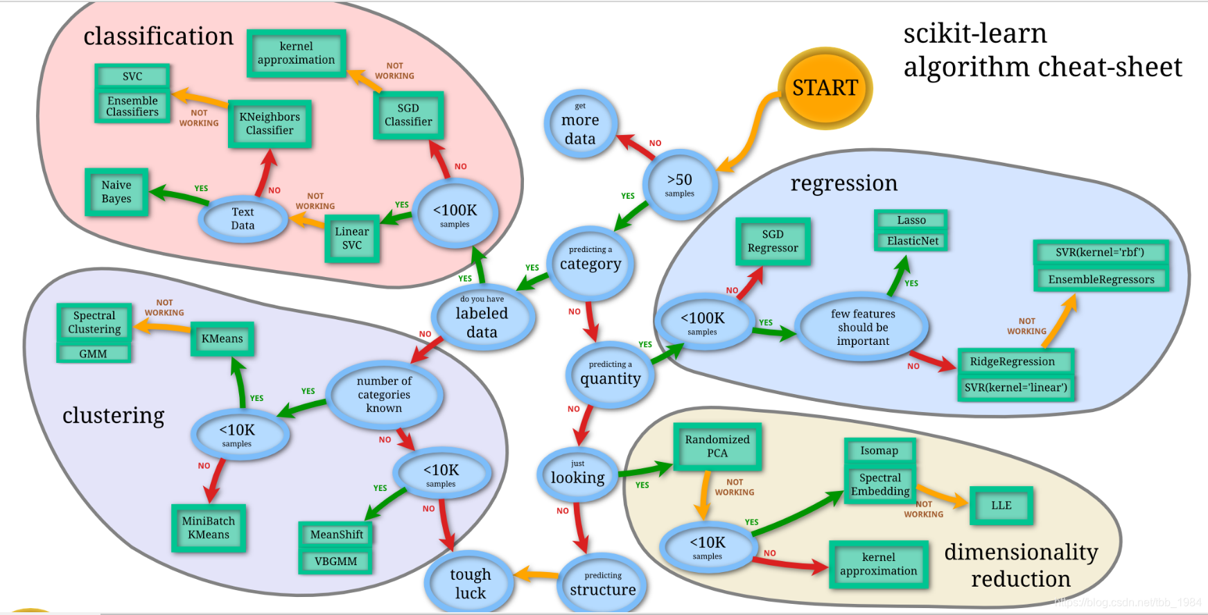
scikit-learn 实现线性回归

SciKit learn的简称是SKlearn，是一个python库，专门用于机器学习的模块。SKlearn包含的机器学习方式： 
分类，回归，无监督，数据降维，数据预处理等等，包含了常见的大部分机器学习方法。

 

x = np.array(X[:, 1].A1)
f = model.predict(X).flatten()

fig, ax = plt.subplots(figsize=(12,8))
ax.plot(x, f, 'r', label='Prediction')
ax.scatter(data.Population, data.Profit, label='Traning Data')
ax.legend(loc=2)
ax.set_xlabel('Population')
ax.set_ylabel('Profit')
ax.set_title('Predicted Profit vs. Population Size')
plt.show()

 normal equation（正规方程）

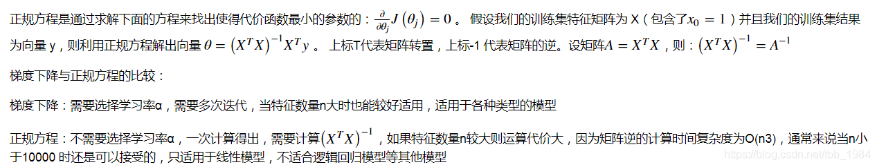
# 正规方程
def normalEqn(X, y):
    theta = np.linalg.inv(X.T@X)@X.T@y#X.T@X等价于X.T.dot(X)
    return theta

 

final_theta2=normalEqn(X, y)
final_theta2