


1.低阶API示范
下面的范例使用TensorFlow的低阶API实现线性回归模型和DNN二分类模型。
import tensorflow as tf
import numpy as np
import pandas as pd
from matplotlib import pyplot as plt
#打印时间分割线
@tf.function
def printbar():
today_ts=tf.timestamp()%(24*60*60)
hour=tf.cast(today_ts//3600+8,tf.int32)%tf.constant(24)
minite=tf.cast((today_ts%3600)//60,tf.int32)
second=tf.cast(tf.floor(today_ts%60),tf.int32)
def timeformat(m):
if tf.strings.length(tf.strings.format("{}",m))==1:
return(tf.strings.format("0{}",m))
else:
return(tf.strings.format("{}",m))
timestring=tf.strings.join([timeformat(hour),timeformat(minite),timeformat(second)],separator=":")
tf.print("=========="*8+timestring)
#准备数据
n=400
#生成测试用数据集
x=tf.random.uniform([n,2],minval=-10,maxval=10)
w0=tf.constant([[2.0],[3.0]])
b0=tf.constant([[3.0]])
y=x@w0+b0+tf.random.normal([n,1],mean=0.0,stddev=2.0)
#@表示矩阵乘法
#数据可视化
def draw_data():
plt.figure(figsize=(12,5))
ax1=plt.subplot(121)
ax1.scatter(x[:,0],y[:,0],c="b")
plt.xlabel("x1")
plt.ylabel("y",rotation=0)
ax1=plt.subplot(122)
ax1.scatter(x[:,1],y[:,0],c="b")
plt.xlabel("x2")
plt.ylabel("y",rotation=0)
plt.show()
draw_data()
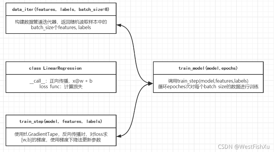
#构建数据管道迭代器
def data_iter(features,labels,batch_size=8):
num_examples=len(features)
indices=list(range(num_examples))
np.random.shuffle(indices)#随机读取样本
for i in range(0,num_examples,batch_size):
indexs=indices[i:min(i+batch_size,num_examples)]
yield tf.gather(features,indexs),tf.gather(labels,indexs)
# tf.gather(params,indices,axis=0 )
# 从params的axis维根据indices的参数值获取切片
#测试数据管道效果
batch_size=8
#next() 返回迭代器的下一个项目。
(features,labels)=next(data_iter(x,y,batch_size))
print(features)
print(labels)
#定义模型
w=tf.Variable(tf.random.normal(w0.shape))
b=tf.Variable(tf.zeros_like(b0,dtype=tf.float32))
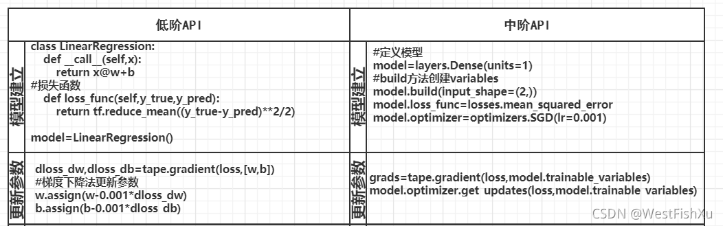
class LinearRegression:
def __call__(self,x):
return x@w+b
#损失函数
def loss_func(self,y_true,y_pred):
return tf.reduce_mean((y_true-y_pred)**2/2)
model=LinearRegression()
#训练模型
def train_step(model,features,labels):
with tf.GradientTape() as tape:
predictions=model(features)
loss=model.loss_func(labels,predictions)
#反向传播求梯度
dloss_dw,dloss_db=tape.gradient(loss,[w,b])
#梯度下降法更新参数
w.assign(w-0.001*dloss_dw)
b.assign(b-0.001*dloss_db)
return loss
#测试train_step
batch_size=10
(features,labels)=next(data_iter(x,y,batch_size))
train_step(model,features,labels)
def train_model(model,epoches):
for epoch in range(1,epoches+1):
for features,labels in data_iter(x,y,10):
loss=train_step(model,features,labels)
if epoch%50==0:
printbar()
tf.print("epoch=",epoch,"loss=",loss)
tf.print("w=",w)
tf.print("b=",b)
train_model(model,epoches=200)
2.中阶API示范
TensorFlow的中阶API主要包括各种模型层,损失函数,优化器,数据管道,特征列等等。
2.1.线性回归模型:
import tensorflow as tf
import numpy as np
import pandas as pd
from matplotlib import pyplot as plt
from tensorflow.python.keras import layers,losses,metrics,optimizers

#打印时间分割线
@tf.function
def printbar():
    today_ts=tf.timestamp()%(24*60*60)

    hour=tf.cast(today_ts//3600+8,tf.int32)%tf.constant(24)
    minite=tf.cast((today_ts%3600)//60,tf.int32)
    second=tf.cast(tf.floor(today_ts%60),tf.int32)

    def timeformat(m):
        if tf.strings.length(tf.strings.format("{}",m))==1:
            return(tf.strings.format("0{}",m))
        else:
            return(tf.strings.format("{}",m))

    timestring=tf.strings.join([timeformat(hour),timeformat(minite),timeformat(second)],separator=":")
    tf.print("=========="*6+timestring)

#样本数量
n=400

#生成测试用数据集
x=tf.random.uniform([n,2],minval=-10,maxval=10)
w0=tf.constant([[2.0],[3.0]])
b0=tf.constant([[3.0]])
y=x@w0+b0+tf.random.normal([n,1],mean=0.0,stddev=2.0)

#构建输入数据管道
def data_iter(features,labels,batch_size=10):
    num_examples=len(features)
    indices=list(range(num_examples))
    np.random.shuffle(indices)#随机读取样本
    for i in range(0,num_examples,batch_size):
        indexs=indices[i:min(i+batch_size,num_examples)]
        yield tf.gather(features,indexs),tf.gather(labels,indexs)
        # tf.gather(params,indices,axis=0 )
        # 从params的axis维根据indices的参数值获取切片

#定义模型
model=layers.Dense(units=1)
#build方法创建variables
model.build(input_shape=(2,))
model.loss_func=losses.mean_squared_error
model.optimizer=optimizers.SGD(lr=0.001)

#使用autograph机制转换成静态图加速
@tf.function
def train_step(model,features,labels):
    with tf.GradientTape() as tape:
        predictions=model(features)
        #其中的-1表示“目前我不确定”
        loss=model.loss_func(tf.reshape(labels,[-1]),tf.reshape(predictions,[-1]))
    grads=tape.gradient(loss,model.trainable_variables)
    model.optimizer.get_updates(loss,model.trainable_variables)
    return loss

#测试train_step效果
#ds是数据输入管道

features,labels=next(data_iter(x,y,batch_size=10))
loss=train_step(model,features,labels)
print("original loss:",loss)

def train_model(model,epoches):
    for epoch in range(1,epoches+1):
        loss=tf.constant(0.0)
        for features,labels in data_iter(x,y,batch_size=10):
            loss=train_step(model,features,labels)
        if epoch%50==0:
            printbar()
            tf.print("epoch =",epoch,"loss = ",loss)
            tf.print("w =",model.variables[0])
            tf.print("b =",model.variables[1])

train_model(model,epoches=200)
2.2.DNN模型
import numpy as np
import pandas as pd
from matplotlib import pyplot as plt
import tensorflow as tf
from tensorflow.python.keras import layers,losses,metrics,optimizers

#打印时间分割线
@tf.function
def printbar():
    today_ts=tf.timestamp()%(24*60*60)

    hour=tf.cast(today_ts//3600+8,tf.int32)%tf.constant(24)
    minite=tf.cast((today_ts%3600)//60,tf.int32)
    second=tf.cast(tf.floor(today_ts%60),tf.int32)

    def timeformat(m):
        if tf.strings.length(tf.strings.format("{}",m))==1:
            return(tf.strings.format("0{}",m))
        else:
            return(tf.strings.format("{}",m))

    timestring=tf.strings.join([timeformat(hour),timeformat(minite),timeformat(second)],separator=":")
    tf.print("=========="*6+timestring)

#正负样本数量
n_positive,n_negative=2000,2000

#生成正负样本
#生成正样本, 小圆环分布
r_p = 5.0 + tf.random.truncated_normal([n_positive,1],0.0,1.0)
theta_p = tf.random.uniform([n_positive,1],0.0,2*np.pi)
xp = tf.concat([r_p*tf.cos(theta_p),r_p*tf.sin(theta_p)],axis = 1)
yp = tf.ones_like(r_p)

#生成负样本, 大圆环分布
r_n = 8.0 + tf.random.truncated_normal([n_negative,1],0.0,1.0)
theta_n = tf.random.uniform([n_negative,1],0.0,2*np.pi)
xn = tf.concat([r_n*tf.cos(theta_n),r_n*tf.sin(theta_n)],axis = 1)
yn = tf.zeros_like(r_n)

#汇总样本
x = tf.concat([xp,xn],axis = 0)
y = tf.concat([yp,yn],axis = 0)

#构建输入数据管道
def data_iter(features,labels,batch_size=10):
    num_examples=len(features)
    indices=list(range(num_examples))
    np.random.shuffle(indices)#随机读取样本
    for i in range(0,num_examples,batch_size):
        indexs=indices[i:min(i+batch_size,num_examples)]
        yield tf.gather(features,indexs),tf.gather(labels,indexs)
        # tf.gather(params,indices,axis=0 )
        # 从params的axis维根据indices的参数值获取切片

#构建输入数据管道
ds = tf.data.Dataset.from_tensor_slices((x,y)) \
     .shuffle(buffer_size = 4000).batch(100) \
     .prefetch(tf.data.experimental.AUTOTUNE)

class DNNModel(tf.Module):
    def __init__(self,name=None):
        super(DNNModel,self).__init__(name=name)
        self.dense1=layers.Dense(4,activation="relu")
        self.dense2=layers.Dense(8,activation="relu")
        self.dense3=layers.Dense(1,activation="sigmoid")

    #正向传播
    @tf.function(input_signature=[tf.TensorSpec(shape = [None,2], dtype = tf.float32)])
    def __call__(self,x):
        x=self.dense1(x)
        x=self.dense2(x)
        y=self.dense3(x)
        return y

model=DNNModel()
model.loss_func=losses.binary_crossentropy
model.metric_func=metrics.binary_accuracy
model.optimizer=optimizers.Adam(lr=0.001)

#测试模型结构
(features,labels)=next(iter(ds))
predictions=model(features)
loss=model.loss_func(tf.reshape(labels,[-1]),tf.reshape(predictions,[-1]))
metric=model.metric_func(tf.reshape(labels,[-1]),tf.reshape(predictions,[-1]))

tf.print("init loss:",loss)
tf.print("init metric",metric)

#使用autograph机制转换成静态图加速
@tf.function
def train_step(model,features,labels):
    predictions=model(features)
    loss=model.loss_func(tf.reshape(labels,[-1]),tf.reshape(predictions,[-1]))
    model.optimizer.get_updates(loss,model.trainable_variables)

    metric=model.metric_func(tf.reshape(labels,[-1]),tf.reshape(predictions,[-1]))

    return loss,metric

def train_model(model,epoches):
    for epoch in range(1,epoches+1):
        loss,metric=tf.constant(0.0),tf.constant(0.0)
        for features,labels in ds:
            loss,metric=train_step(model,features,labels)
        if epoch%10==0:
            printbar()
            tf.print("epoch =",epoch,"loss = ",loss, "accuracy = ",metric)
train_model(model,epoches = 100)


# 结果可视化
fig, (ax1,ax2) = plt.subplots(nrows=1,ncols=2,figsize = (12,5))
ax1.scatter(xp[:,0].numpy(),xp[:,1].numpy(),c = "r")
ax1.scatter(xn[:,0].numpy(),xn[:,1].numpy(),c = "g")
ax1.legend(["positive","negative"]);
ax1.set_title("y_true");

xp_pred = tf.boolean_mask(x,tf.squeeze(model(x)>=0.5),axis = 0)
xn_pred = tf.boolean_mask(x,tf.squeeze(model(x)<0.5),axis = 0)

ax2.scatter(xp_pred[:,0].numpy(),xp_pred[:,1].numpy(),c = "r")
ax2.scatter(xn_pred[:,0].numpy(),xn_pred[:,1].numpy(),c = "g")
ax2.legend(["positive","negative"]);
ax2.set_title("y_pred");
plt.show()
3.高阶API示范
TensorFlow的高阶API主要为tf.keras.models提供的模型的类接口
使用Keras接口有以下3种方式构建模型:使用Sequential按层顺序构建模型,使用函数式API构建任意结构模型,继承Model基类构建自定义模型。
此处分别演示使用Sequential按层顺序构建模型以及继承Model基类构建自定义模型。
3.1.线性回归
使用Sequential按层顺序构建模型
`import tensorflow as tf
import numpy as np
import pandas as pd
from matplotlib import pyplot as plt
import tensorflow as tf
from tensorflow.keras import models,layers,losses,metrics,optimizers
#打印时间分割线
@tf.function
def printbar():
today_ts = tf.timestamp()%(24*60*60)
hour = tf.cast(today_ts//3600+8,tf.int32)%tf.constant(24)
minite = tf.cast((today_ts%3600)//60,tf.int32)
second = tf.cast(tf.floor(today_ts%60),tf.int32)
def timeformat(m):
if tf.strings.length(tf.strings.format("{}",m))==1:
return(tf.strings.format("0{}",m))
else:
return(tf.strings.format("{}",m))
timestring = tf.strings.join([timeformat(hour),timeformat(minite),
timeformat(second)],separator = ":")
tf.print("=========="*8+timestring)
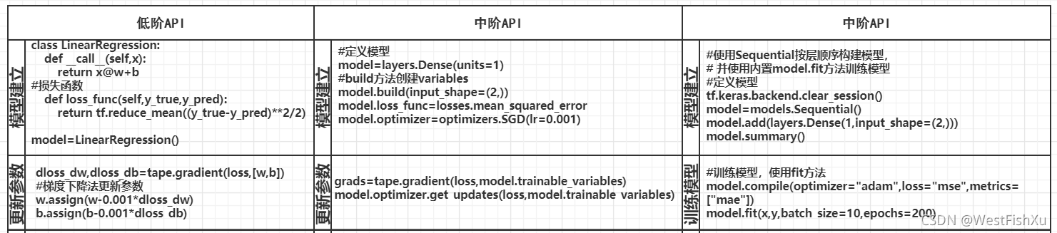
#使用Sequential按层顺序构建模型,
# 并使用内置model.fit方法训练模型
#准备数据
n=400
#生成测试用数据集
x=tf.random.uniform([n,2],minval=-10,maxval=10)
w0=tf.constant([[2.0],[3.0]])
b0=tf.constant([[3.0]])
y=x@w0+b0+tf.random.normal([n,1],mean=0.0,stddev=2.0)
#定义模型
tf.keras.backend.clear_session()
model=models.Sequential()
model.add(layers.Dense(1,input_shape=(2,)))
model.summary()
#训练模型,使用fit方法
model.compile(optimizer="adam",loss="mse",metrics=["mae"])
model.fit(x,y,batch_size=10,epochs=200)
tf.print("w = ",model.layers[0].kernel)
tf.print("b = ",model.layers[0].bias)`
3.2.DNN二分模型
继承Model基类构建自定义模型
import numpy as np
import pandas as pd
from matplotlib import pyplot as plt
import tensorflow as tf
from tensorflow.keras import models,layers,losses,metrics,optimizers

n=400
#打印时间分割线
@tf.function
def printbar():
    today_ts=tf.timestamp()%(24*60*60)

    hour=tf.cast(today_ts//3600+8,tf.int32)%tf.constant(24)
    minite=tf.cast((today_ts%3600)//60,tf.int32)
    second=tf.cast(tf.floor(today_ts%60),tf.int32)

    def timeformat(m):
        if tf.strings.length(tf.strings.format("{}",m))==1:
            return(tf.strings.format("0{}",m))
        else:
            return(tf.strings.format("{}",m))

    timestring=tf.strings.join([timeformat(hour),timeformat(minite),timeformat(second)],separator=":")
    tf.print("=========="*8+timestring)

n_positive,n_negative=2000,2000

#生成正样本
r_p=5.0+tf.random.truncated_normal([n_positive,1],0.0,1.0)
theta_p=tf.random.uniform([n_positive,1],0.0,2*np.pi)
xp=tf.concat([r_p*tf.cos(theta_p),r_p*tf.sin(theta_p)],axis=1)
yp=tf.ones_like(r_p)

#生成负样本
r_n=8.0+tf.random.truncated_normal([n_negative,1],0.0,1.0)
theta_n=tf.random.uniform([n_negative,1],0.0,2*np.pi)
xn=tf.concat([r_n*tf.cos(theta_n),r_n*tf.sin(theta_n)],axis=1)
yn=tf.zeros_like(r_n)

#汇总样本
#x是n_negative行2列
x=tf.concat([xp,xn],axis=0)
y=tf.concat([yp,yn],axis=0)
#样本洗牌
#data是n_negative行3列
data=tf.concat([x,y],axis=1)
#随机地将张量沿其第一维度打乱.也就是列不变,行之间打乱
data=tf.random.shuffle(data)
x=data[:,:2]
y=data[:,2:]

#数据可视化
def draw_data():
    plt.figure(figsize=(6,6))
    plt.scatter(xp[:,0].numpy(),xp[:,1].numpy(),c='r')
    plt.scatter(xn[:,0].numpy(),xn[:,1].numpy(),c='g')
    plt.legend(['positive','negative'])
    plt.show()

#draw_data()
#数据抽取,分为测试集和训练集
ds_train=tf.data.Dataset.from_tensor_slices((x[0:n*3//4,:],y[0:n*3//4,:])) \
    .shuffle(buffer_size = 1000).batch(20) \
        .prefetch(tf.data.experimental.AUTOTUNE) \
            .cache()
ds_valid = tf.data.Dataset.from_tensor_slices((x[n*3//4:,:],y[n*3//4:,:])) \
    .batch(20) \
        .prefetch(tf.data.experimental.AUTOTUNE) \
            .cache()

#定义模型
tf.keras.backend.clear_session()
class DNNModel(models.Model):
    def __init__(self):
        super(DNNModel,self).__init__()

    def build(self,input_shape):
        #inputs:输入该网络层的数据
        #units=4、8、1:输出的维度大小,改变inputs的最后一维
        self.dense1 = layers.Dense(4,activation = "relu",name = "dense1")
        self.dense2 = layers.Dense(8,activation = "relu",name = "dense2")
        self.dense3 = layers.Dense(1,activation = "sigmoid",name = "dense3")
        super(DNNModel,self).build(input_shape)

    #正向传播
    @tf.function(input_signature=[tf.TensorSpec(shape = [None,2], dtype = tf.float32)])
    def call(self,x):
        x=self.dense1(x)
        x=self.dense2(x)
        y=self.dense3(x)
        return y

model=DNNModel()
model.build(input_shape=(None,2))
#关于参数个数的计算:
#dense1:输入两列数据,输出为4个单元
model.summary()

#自定义训练循环

optimizer=optimizers.Adam(lr=0.001)
loss_func=tf.keras.losses.BinaryCrossentropy()
#train_loss是训练数据上的损失,衡量模型在训练集上的拟合能力。
#valid_loss是在验证集上的损失,衡量的是在未见过数据上的拟合能力
train_loss=tf.keras.metrics.Mean(name='train_loss')
train_metric=tf.keras.metrics.BinaryAccuracy(name='train_accuracy')

valid_loss=tf.keras.metrics.Mean(name='valid_loss')
valid_metric=tf.keras.metrics.BinaryAccuracy(name='valid_accuracy')
#训练集的train需要更新参数optimizer.get_updates(loss,model.trainable_variables)
@tf.function
def train_step(model,features,labels):
    predictions=model(features)
    loss=loss_func(labels,predictions)
    optimizer.get_updates(loss,model.trainable_variables)
    train_loss.update_state(loss)
    train_metric.update_state(labels,predictions)
#测试集的不需要更新参数,只是需要计算loss和metric
@tf.function
def valid_step(model,features,labels):
    predictions=model(features)
    batch_loss=loss_func(labels,predictions)
    valid_loss.update_state(batch_loss)
    valid_metric.update_state(labels,predictions)
#update_state(),将每一次更新的数据作为一组数据,在真正计算的时候会计算出每一组的结果,
# 然后求多组结果的平均值。但并不会直接计算,计算还是在调用 result()时完成
def train_model(model,ds_train,ds_valid,epochs):
    for epoch in range(1,epochs+1):
        for features,labels in ds_train:
            train_step(model,features,labels)

        for features,labels in ds_valid:
            valid_step(model,features,labels)

        logs='Epoch={},Loss:{},Accuracy:{},Valid Loss:{},Valid Accuracy:{}'
        if  epoch%100 ==0:
            printbar()
            tf.print(tf.strings.format(logs,(epoch,train_loss.result(),train_metric.result(),valid_loss.result(),valid_metric.result())))

        train_loss.reset_states()
        valid_loss.reset_states()
        train_metric.reset_states()
        valid_metric.reset_states()

train_model(model,ds_train,ds_valid,1000)


 4894
4894

 被折叠的 条评论
为什么被折叠?
被折叠的 条评论
为什么被折叠?
 到【灌水乐园】发言


